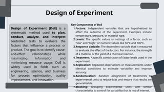
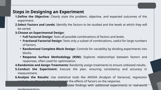
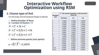
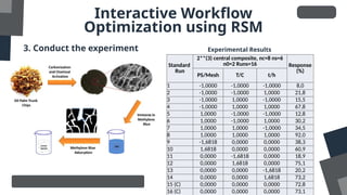
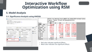
TIBCO Statistica
OPTIMIZATION
USING RSM
Universitas Diponegoro | Faculty of Engineering | 2024
By: Dani Puji Utomo
Department of Chemical Engineering
DAFTAR ISI
Design of Experiment (DOE)
Optimization Method
Introduction of RSM
TIBCO Statistica
DOE using Statistica
RSM Optimization using Statistica
01
02
03
04
05
06
Design of Experiment (DoE) is a
systematic method used to plan,
conduct, analyze, and interpret
controlled tests to evaluate the
factors that influence a process or
product. The goal is to identify cause-
and-effect relationships while
maximizing information and
minimizing resource usage. DoE is
widely used in fields such as
engineering, science, and business
for process optimization, quality
improvement, and innovation.
Design of Experiment
Key Components of DoE
1.Factors: Independent variables that are hypothesized to
affect the outcome of the experiment. Examples include
temperature, pressure, or material type.
2.Levels: The specific values or settings of a factor, such as
"low" and "high," or numeric values like 50°C and 100°C.
3.Response Variable: The dependent variable that is measured
to evaluate the effect of the factors. For instance, the strength
of a material or the yield of a chemical reaction.
4.Treatment: A specific combination of factor levels used in the
experiment.
5.Replication: Repeated observations or measurements under
identical conditions to estimate variability and improve
accuracy.
6.Randomization: Random assignment of treatments to
experimental units to reduce bias and ensure that results are
generalizable.
7.Blocking: Grouping experimental units with similar
characteristics to control for variability that is not of interest.
Steps in Designing an Experiment
1.Define the Objective: Clearly state the problem, objective, and expected outcomes of the
experiment.
2.Select Factors and Levels: Identify the factors to be studied and the levels at which they will
be varied.
3.Choose an Experimental Design:
⚬ Full Factorial Design: Tests all possible combinations of factors and levels.
⚬ Fractional Factorial Design: Tests only a subset of combinations, useful for large numbers
of factors.
⚬ Randomized Complete Block Design: Controls for variability by dividing experiments into
blocks.
⚬ Response Surface Methodology (RSM): Explores relationships between factors and
responses, often used for optimization.
4.Randomize and Assign Treatments: Randomly assign treatments to ensure unbiased results.
5.Conduct the Experiment: Execute the plan, ensuring consistency and accuracy in
measurement.
6.Analyze the Results: Use statistical tools like ANOVA (Analysis of Variance), regression
analysis, or other models to interpret the effects of factors on the response.
7.Draw Conclusions and Verify: Validate findings with additional experiments or real-world
Full Factorial Design
Full Factorial Design is an experimental design method where all possible
combinations of the levels of factors are tested. This approach allows for a thorough
examination of the individual effects of each factor as well as the interactions between
factors. It is often considered the "gold standard" for experiments when the goal is to
gain complete understanding of the system being studied.
Commonly represented as k ,
where:
k = number of levels for each
factor.
n = number of factors.
n Example of a 2-Level Full Factorial Design
Consider an experiment with 2 factors:
• Factor A: Temperature (low, high)
• Factor B: Pressure (low, high)
Each factor has 2 levels. A full factorial design includes 2^2 =4
runs:
1.Low Temperature, Low Pressure
2.Low Temperature, High Pressure
3.High Temperature, Low Pressure
4.High Temperature, High Pressure
Fractional Factorial Design
Fractional Factorial Design is a variation of the Full Factorial Design that reduces the
number of experimental runs by only testing a selected subset of all possible
combinations of factor levels. It is particularly useful when a full factorial experiment is
impractical due to time, cost, or resource constraints, especially with a large number of
factors.
fractional factorial design may
involve a 2 subset:
• p : The fraction of runs
omitted.
• 2 : The number of runs
conducted.
k−
p
k−
p
Randomized Complete Block Design
Randomized Complete Block Design (RCBD) is an experimental design used to control
for variability among experimental units by grouping them into blocks based on certain
characteristics that might influence the response variable. Within each block, treatments
are randomly assigned to the experimental units, ensuring that the comparison
between treatments is not confounded by block effects.
Key Features of RCBD
• Blocking: Experimental units are divided into blocks based on known sources of variability (e.g.,
location, time, or other conditions). Each block should contain experimental units that are as
similar as possible.
• Randomization: reatments are randomly assigned within each block to eliminate bias.
• Completeness: Every block contains all treatments, ensuring that each treatment is tested under
similar conditions.
• Control for Variability: Variability between blocks is accounted for, improving the precision of the
treatment effect estimation.
Response Surface
Method
Response Surface Methodology (RSM) is a set of statistical and mathematical
techniques used to model and analyze problems where a response (dependent variable)
is influenced by several factors (independent variables). The goal is to optimize the
response by finding the best levels of the factors. RSM is particularly useful in situations
where there is a need to fine-tune a process or product.
Design Types in RSM
1. Central Composite Design (CCD):
• Most commonly used RSM design.
• Combines a factorial design, center points, and axial
points.
• Allows for the estimation of quadratic effects.
2. Box-Behnken Design (BBD):
• Does not include extreme (axial) points.
• Useful for experiments where the range of factor
levels is limited.
• Requires fewer runs compared to CCD.
3. Doehlert Design:
• Efficient for experiments with a high number of
factors.
• Ensures uniform precision over the experimental
space.
4. Face-Centered Central Composite Design
(FCCCD):
• A variation of CCD where axial points are located
on the faces of the factorial cube.
5. Mixture Design
• ‘In a mixture design, the sum of the component
proportions is always fixed
Central Composite
Design (CCD)
To maintain rotatability, the value of α depends on the
number of experimental runs in the factorial portion of the
central composite design:
If the factorial is a full factorial,
then
  
1
4
factorial run
 
 
1
4
2k
  
 
Then, the number of experimental runs:
2 2
k
N k C
  
where:
• 𝑘 is the number of factors,
• 𝐶 is the number of center points (which is optional but
typically included for increased model reliability).
Types of CCD
Type of CCD Description Key Features
Circumscribed CCD (CCC)
The most traditional form
of CCD where axial points
lie outside the cube
(factorial region).
- Axial (star) points are at a
distance ±α from the
center.
- α is determined by
rotatability or
orthogonality.
Inscribed CCD (CCI)
A scaled-down version of
CCC where the factorial
points lie within the
feasible region defined by
the experiment.
- Axial points are located
inside the cube.
- Used when factor levels
must be restricted to a
safe or feasible range.
Face-Centered CCD (FCC)
A version of CCD where
the axial points are placed
at the center of each face
of the factorial cube.
- Axial points are at a
distance of ±1 from the
center.
- Does not extend beyond
the factorial region.
Box-Behnken Design
(BBD)
Box-Behnken Design (BBD) is a type of experimental design used in Response
Surface Methodology (RSM) to explore the relationships between several explanatory
variables and a response variable. It is particularly useful for optimizing processes and
finding optimal settings for variables with fewer experimental runs compared to
traditional designs, such as full factorial designs.
 
2 1
N k k C
  
where:
• 𝑘 is the number of factors,
• 𝐶 is the number of center points (which is optional but
typically included for increased model reliability).
The experimental runs are designed using combinations of three levels for
each factor, but there are no combinations at the extremes of the factor
space. This results in a spherical or circular design structure.
In a Box-Behnken design for k factors, the experimental runs are
arranged as follows:
• The design includes factorial points and center points.
• There are no corner points (i.e., the extreme values for all factors
simultaneously).
• The runs are arranged so that each factor is varied at low, medium,
and high levels.
Optimization using RSM
Optimization in RSM refers to finding the input values (or factor settings) that
result in the best possible outcome (response), typically by maximizing or
minimizing a certain response variable.
Response Surface Methodology (RSM) is a collection of mathematical and
statistical techniques used to model and analyze the relationship between a
response variable and multiple input (predictor) variables. It is primarily used for
optimizing processes, improving product quality, and identifying optimal factor
settings in a system.
Typically, a second-order polynomial model is used, which includes linear,
interaction, and quadratic terms:
2 2 2
0 1 1 2 2 3 3 12 1 2 13 1 3 23 2 3 11 1 22 2 33 3
Y X X X X X X X X X X X X
         
          
Where:
• Y is the response variable
• X1, X2, X3​are the factors (independent variables),
• β0, β1, β2,… are the regression coefficients,
• ϵ is the error term.
Steps in Optimization using RSM
Tools in Optimization using RSM
TIBCO Statistica®
is a flexible analytics system, which allows users to, create analytic
workflows that are packaged and published to business users, explore interactively
and visualize, create and deploy statistical, predictive, data mining, machine learning,
forecasting, optimization, and text analytic models.
Latest Version : TIBCO Statistica™ 14.0.0
Design–Expert is a statistical software package from Stat-Ease Inc. that is specifically
dedicated to performing design of experiments (DOE). Design–Expert offers
comparative tests, screening, characterization, optimization, robust parameter
design, mixture designs and combined designs.
Latest Version: Design-Expert v23.1
JASP (Jeffreys’s Amazing Statistics Program) is a free and open-source program
for statistical analysis supported by the University of Amsterdam. It is designed to be
easy to use, and familiar to users of SPSS.
Latest Version: JASP 0.19.1.
User Interface TIBCO Statistica
Interactive Workflow
Optimization using RSM
1. Define The Problem
Optimization of adsorption capacity of Elaeis
guineensis-activated carbon for methylene blue
removal
Factors with coded value
Factors Low Level Mid Level High Level
Particle size (Mesh) 32 48 64
Temperature (C) 500 600 700
Time (h) 1 2 3
Response:
 
0
0
% 100%
t
C C
removal
C

 
In this equation,
• C0 are the solution concentrations at initial (mg/L)
• Ct are the solution concentration at time t (mg/L)
Factors Low Level Mid Level High Level
Particle size (Mesh) -1 0 1
Temperature (C) -1 0 1
Time (h) -1 0 1
 
0
i i
i
i
X X
x
X



Factors with original value
In this equation,
• xi is the coded value of ith
factors / independent
variables
• Xi is original value of ith
factors
• Xi
0
is original value of center point
• ΔXi is the difference between maximum and
Interactive Workflow
Optimization using RSM
2. Choose type of DoE
For this study, Central Composite Design is selected
• Define Number of Runs
k = number of factors = 3
2 2
k
N k C
  
3
3
2 2(3) 2 16
2 2(3) 3 17
N
N
   
   
• Define extreme points (star points)
 
1
4
2 1,6818
k
  
Standard
Run
2**(3) central composite, nc=8 ns=6 n0=2
Runs=16
PS/Mesh T/C t/h
1 -1,0000 -1,0000 -1,0000
2 -1,0000 -1,0000 1,0000
3 -1,0000 1,0000 -1,0000
4 -1,0000 1,0000 1,0000
5 1,0000 -1,0000 -1,0000
6 1,0000 -1,0000 1,0000
7 1,0000 1,0000 -1,0000
8 1,0000 1,0000 1,0000
9 -1,6818 0,0000 0,0000
10 1,6818 0,0000 0,0000
11 0,0000 -1,6818 0,0000
12 0,0000 1,6818 0,0000
13 0,0000 0,0000 -1,6818
14 0,0000 0,0000 1,6818
15 (C) 0,0000 0,0000 0,0000
16 (C) 0,0000 0,0000 0,0000
Interactive Workflow
Optimization using RSM
3. Conduct the experiment
Standard
Run
2**(3) central composite, nc=8 ns=6
n0=2 Runs=16 Response
(%)
PS/Mesh T/C t/h
1 -1,0000 -1,0000 -1,0000 8,0
2 -1,0000 -1,0000 1,0000 21,8
3 -1,0000 1,0000 -1,0000 15,5
4 -1,0000 1,0000 1,0000 67,8
5 1,0000 -1,0000 -1,0000 12,8
6 1,0000 -1,0000 1,0000 30,2
7 1,0000 1,0000 -1,0000 34,5
8 1,0000 1,0000 1,0000 92,0
9 -1,6818 0,0000 0,0000 38,3
10 1,6818 0,0000 0,0000 60,9
11 0,0000 -1,6818 0,0000 18,9
12 0,0000 1,6818 0,0000 75,1
13 0,0000 0,0000 -1,6818 20,2
14 0,0000 0,0000 1,6818 73,2
15 (C) 0,0000 0,0000 0,0000 72,8
16 (C) 0,0000 0,0000 0,0000 73,1
Experimental Results
Interactive Workflow
Optimization using RSM
4. Fitting Model
2 2 2
1 2 3 1 2 3
1 2 1 3 2 3
74,00 6,91 16,95 16,85 10,80 11,72 11,82
3,75 1,10 9,82
Y X X X X X X
X X X X X X
      
  
2 1
0
1 1 1
n n n n
i i i i ij i j
i i i j
Y x x x x
   

  
 
    
 
 
   
Interactive Workflow
Optimization using RSM
5. Model Analysis
5.1. Significance Analysis using ANOVA
a. Formulate the hypotheses
• Null Hypothesis = The model has no significant effect on the response
• Alternative Hypothesis: The model has significant effect on the response
b. Sum of Squares
• Total Sum of Squares (SST): Measures the total variability in the response variable.
• Regression Sum of Squares (SSR): Measures the variability explained by the model.
• Residual Sum of Squares (SSE): Measures the variability due to random error or unexplained
variation
c. Mean of Squares
• Mean Square for Regression (MSR): MSR=SSR/p with p is the number of model parameters
• Mean Square for Error (MSE): MSE= SSE/(n-p-1)​, where n is the total number of data points.
d. F-test
• The F-statistic is calculated by dividing the mean square for regression (MSR) by the mean
square for error (MSE)
d. p-value
• A low p-value (typically p<0.05) indicates that the model is statistically significant)
Interactive Workflow
Optimization using RSM
5. Model Analysis
5.1. Significance Analysis using ANOVA
• Red color indicates significant Effects
• Black color indicates non significant Effects
Interactive Workflow
Optimization using RSM
5. Model Analysis
5.1. Significance Analysis using ANOVA
Interactive Workflow
Optimization using RSM
5. Model Analysis
5.2. Model Adequacy Check
• R2
= 0,9666
• Adj-R2
= 0,9165
Interactive Workflow
Optimization using RSM
6. Optimize the Model
6.1 Single Response Optimization 6.2 Multiple Responses Optimization
(later)
• Put value 0 desirability for
undesired level value
• Put value 1 desirability for
desired level value
Suitable for optimizing
multiple responses with trade-
off profile,
for example in maximizing the
Yield and minimizing
Production Cost
Optimized Value
• PS =
0,6255
• Temp = 1,3738
• Time = 1,3125
Interactive Workflow
Optimization using RSM
6. Optimize the Model
6.3 Surface and Contour Plot
Interactive Workflow
Optimization using RSM
6. Verification
Conduct experimental verification
Optimized Value  Convert to original
value
• PS = 0,6255
• Temp = 1,3738
• Time = 1,3125
0
i i i i
X X x X
 
 
16 0,6255 48 58,01
PS    
 
100 1,3738 600 738
Temp    
 
1 1,3125 2 3,31
Time    
Verif Run Predicted Experiment SSR
Run 1 98,86 98,27 0,3481
Run 2 98,86 97,89 0,9409
Run 3 98,86 99,12 0,0676
Total 1,3566
Error 0,8236
% error 0,83%
Interactive Workflow
Optimization using RSM
6.2 Simultaneous Optimization for Multiple Responses
• From the Prediction & Profiling Tab  Click on Response
Desirability Profiling
• Checklist the show desirability function
• Put value of 0.00; 0.50; and 1.00 for undesired, mid desired, and
very desired value level, respectively
• Set factors at Optimum Value
• You may set the factor grid by approximately 20 steps
• Click View to show the compound desirability optimization
• Click 3D response and contour icons to show the plot
Interactive Workflow
Optimization using RSM
The Optimum Value for Desired Response
Interactive Workflow
Optimization using RSM
3D Surface and Contour Compound Plot
Optimization using RSM TIBCO Statistica.pptx

Optimization using RSM TIBCO Statistica.pptx

  • 1.
    TIBCO Statistica OPTIMIZATION USING RSM UniversitasDiponegoro | Faculty of Engineering | 2024 By: Dani Puji Utomo Department of Chemical Engineering
  • 2.
    DAFTAR ISI Design ofExperiment (DOE) Optimization Method Introduction of RSM TIBCO Statistica DOE using Statistica RSM Optimization using Statistica 01 02 03 04 05 06
  • 3.
    Design of Experiment(DoE) is a systematic method used to plan, conduct, analyze, and interpret controlled tests to evaluate the factors that influence a process or product. The goal is to identify cause- and-effect relationships while maximizing information and minimizing resource usage. DoE is widely used in fields such as engineering, science, and business for process optimization, quality improvement, and innovation. Design of Experiment Key Components of DoE 1.Factors: Independent variables that are hypothesized to affect the outcome of the experiment. Examples include temperature, pressure, or material type. 2.Levels: The specific values or settings of a factor, such as "low" and "high," or numeric values like 50°C and 100°C. 3.Response Variable: The dependent variable that is measured to evaluate the effect of the factors. For instance, the strength of a material or the yield of a chemical reaction. 4.Treatment: A specific combination of factor levels used in the experiment. 5.Replication: Repeated observations or measurements under identical conditions to estimate variability and improve accuracy. 6.Randomization: Random assignment of treatments to experimental units to reduce bias and ensure that results are generalizable. 7.Blocking: Grouping experimental units with similar characteristics to control for variability that is not of interest.
  • 4.
    Steps in Designingan Experiment 1.Define the Objective: Clearly state the problem, objective, and expected outcomes of the experiment. 2.Select Factors and Levels: Identify the factors to be studied and the levels at which they will be varied. 3.Choose an Experimental Design: ⚬ Full Factorial Design: Tests all possible combinations of factors and levels. ⚬ Fractional Factorial Design: Tests only a subset of combinations, useful for large numbers of factors. ⚬ Randomized Complete Block Design: Controls for variability by dividing experiments into blocks. ⚬ Response Surface Methodology (RSM): Explores relationships between factors and responses, often used for optimization. 4.Randomize and Assign Treatments: Randomly assign treatments to ensure unbiased results. 5.Conduct the Experiment: Execute the plan, ensuring consistency and accuracy in measurement. 6.Analyze the Results: Use statistical tools like ANOVA (Analysis of Variance), regression analysis, or other models to interpret the effects of factors on the response. 7.Draw Conclusions and Verify: Validate findings with additional experiments or real-world
  • 5.
    Full Factorial Design FullFactorial Design is an experimental design method where all possible combinations of the levels of factors are tested. This approach allows for a thorough examination of the individual effects of each factor as well as the interactions between factors. It is often considered the "gold standard" for experiments when the goal is to gain complete understanding of the system being studied. Commonly represented as k , where: k = number of levels for each factor. n = number of factors. n Example of a 2-Level Full Factorial Design Consider an experiment with 2 factors: • Factor A: Temperature (low, high) • Factor B: Pressure (low, high) Each factor has 2 levels. A full factorial design includes 2^2 =4 runs: 1.Low Temperature, Low Pressure 2.Low Temperature, High Pressure 3.High Temperature, Low Pressure 4.High Temperature, High Pressure
  • 6.
    Fractional Factorial Design FractionalFactorial Design is a variation of the Full Factorial Design that reduces the number of experimental runs by only testing a selected subset of all possible combinations of factor levels. It is particularly useful when a full factorial experiment is impractical due to time, cost, or resource constraints, especially with a large number of factors. fractional factorial design may involve a 2 subset: • p : The fraction of runs omitted. • 2 : The number of runs conducted. k− p k− p
  • 7.
    Randomized Complete BlockDesign Randomized Complete Block Design (RCBD) is an experimental design used to control for variability among experimental units by grouping them into blocks based on certain characteristics that might influence the response variable. Within each block, treatments are randomly assigned to the experimental units, ensuring that the comparison between treatments is not confounded by block effects. Key Features of RCBD • Blocking: Experimental units are divided into blocks based on known sources of variability (e.g., location, time, or other conditions). Each block should contain experimental units that are as similar as possible. • Randomization: reatments are randomly assigned within each block to eliminate bias. • Completeness: Every block contains all treatments, ensuring that each treatment is tested under similar conditions. • Control for Variability: Variability between blocks is accounted for, improving the precision of the treatment effect estimation.
  • 8.
    Response Surface Method Response SurfaceMethodology (RSM) is a set of statistical and mathematical techniques used to model and analyze problems where a response (dependent variable) is influenced by several factors (independent variables). The goal is to optimize the response by finding the best levels of the factors. RSM is particularly useful in situations where there is a need to fine-tune a process or product. Design Types in RSM 1. Central Composite Design (CCD): • Most commonly used RSM design. • Combines a factorial design, center points, and axial points. • Allows for the estimation of quadratic effects. 2. Box-Behnken Design (BBD): • Does not include extreme (axial) points. • Useful for experiments where the range of factor levels is limited. • Requires fewer runs compared to CCD. 3. Doehlert Design: • Efficient for experiments with a high number of factors. • Ensures uniform precision over the experimental space. 4. Face-Centered Central Composite Design (FCCCD): • A variation of CCD where axial points are located on the faces of the factorial cube. 5. Mixture Design • ‘In a mixture design, the sum of the component proportions is always fixed
  • 9.
    Central Composite Design (CCD) Tomaintain rotatability, the value of α depends on the number of experimental runs in the factorial portion of the central composite design: If the factorial is a full factorial, then    1 4 factorial run     1 4 2k      Then, the number of experimental runs: 2 2 k N k C    where: • 𝑘 is the number of factors, • 𝐶 is the number of center points (which is optional but typically included for increased model reliability).
  • 10.
    Types of CCD Typeof CCD Description Key Features Circumscribed CCD (CCC) The most traditional form of CCD where axial points lie outside the cube (factorial region). - Axial (star) points are at a distance ±α from the center. - α is determined by rotatability or orthogonality. Inscribed CCD (CCI) A scaled-down version of CCC where the factorial points lie within the feasible region defined by the experiment. - Axial points are located inside the cube. - Used when factor levels must be restricted to a safe or feasible range. Face-Centered CCD (FCC) A version of CCD where the axial points are placed at the center of each face of the factorial cube. - Axial points are at a distance of ±1 from the center. - Does not extend beyond the factorial region.
  • 11.
    Box-Behnken Design (BBD) Box-Behnken Design(BBD) is a type of experimental design used in Response Surface Methodology (RSM) to explore the relationships between several explanatory variables and a response variable. It is particularly useful for optimizing processes and finding optimal settings for variables with fewer experimental runs compared to traditional designs, such as full factorial designs.   2 1 N k k C    where: • 𝑘 is the number of factors, • 𝐶 is the number of center points (which is optional but typically included for increased model reliability). The experimental runs are designed using combinations of three levels for each factor, but there are no combinations at the extremes of the factor space. This results in a spherical or circular design structure. In a Box-Behnken design for k factors, the experimental runs are arranged as follows: • The design includes factorial points and center points. • There are no corner points (i.e., the extreme values for all factors simultaneously). • The runs are arranged so that each factor is varied at low, medium, and high levels.
  • 12.
    Optimization using RSM Optimizationin RSM refers to finding the input values (or factor settings) that result in the best possible outcome (response), typically by maximizing or minimizing a certain response variable. Response Surface Methodology (RSM) is a collection of mathematical and statistical techniques used to model and analyze the relationship between a response variable and multiple input (predictor) variables. It is primarily used for optimizing processes, improving product quality, and identifying optimal factor settings in a system. Typically, a second-order polynomial model is used, which includes linear, interaction, and quadratic terms: 2 2 2 0 1 1 2 2 3 3 12 1 2 13 1 3 23 2 3 11 1 22 2 33 3 Y X X X X X X X X X X X X                      Where: • Y is the response variable • X1, X2, X3​are the factors (independent variables), • β0, β1, β2,… are the regression coefficients, • ϵ is the error term.
  • 13.
  • 14.
    Tools in Optimizationusing RSM TIBCO Statistica® is a flexible analytics system, which allows users to, create analytic workflows that are packaged and published to business users, explore interactively and visualize, create and deploy statistical, predictive, data mining, machine learning, forecasting, optimization, and text analytic models. Latest Version : TIBCO Statistica™ 14.0.0 Design–Expert is a statistical software package from Stat-Ease Inc. that is specifically dedicated to performing design of experiments (DOE). Design–Expert offers comparative tests, screening, characterization, optimization, robust parameter design, mixture designs and combined designs. Latest Version: Design-Expert v23.1 JASP (Jeffreys’s Amazing Statistics Program) is a free and open-source program for statistical analysis supported by the University of Amsterdam. It is designed to be easy to use, and familiar to users of SPSS. Latest Version: JASP 0.19.1.
  • 15.
  • 16.
    Interactive Workflow Optimization usingRSM 1. Define The Problem Optimization of adsorption capacity of Elaeis guineensis-activated carbon for methylene blue removal Factors with coded value Factors Low Level Mid Level High Level Particle size (Mesh) 32 48 64 Temperature (C) 500 600 700 Time (h) 1 2 3 Response:   0 0 % 100% t C C removal C    In this equation, • C0 are the solution concentrations at initial (mg/L) • Ct are the solution concentration at time t (mg/L) Factors Low Level Mid Level High Level Particle size (Mesh) -1 0 1 Temperature (C) -1 0 1 Time (h) -1 0 1   0 i i i i X X x X    Factors with original value In this equation, • xi is the coded value of ith factors / independent variables • Xi is original value of ith factors • Xi 0 is original value of center point • ΔXi is the difference between maximum and
  • 17.
    Interactive Workflow Optimization usingRSM 2. Choose type of DoE For this study, Central Composite Design is selected • Define Number of Runs k = number of factors = 3 2 2 k N k C    3 3 2 2(3) 2 16 2 2(3) 3 17 N N         • Define extreme points (star points)   1 4 2 1,6818 k    Standard Run 2**(3) central composite, nc=8 ns=6 n0=2 Runs=16 PS/Mesh T/C t/h 1 -1,0000 -1,0000 -1,0000 2 -1,0000 -1,0000 1,0000 3 -1,0000 1,0000 -1,0000 4 -1,0000 1,0000 1,0000 5 1,0000 -1,0000 -1,0000 6 1,0000 -1,0000 1,0000 7 1,0000 1,0000 -1,0000 8 1,0000 1,0000 1,0000 9 -1,6818 0,0000 0,0000 10 1,6818 0,0000 0,0000 11 0,0000 -1,6818 0,0000 12 0,0000 1,6818 0,0000 13 0,0000 0,0000 -1,6818 14 0,0000 0,0000 1,6818 15 (C) 0,0000 0,0000 0,0000 16 (C) 0,0000 0,0000 0,0000
  • 18.
    Interactive Workflow Optimization usingRSM 3. Conduct the experiment Standard Run 2**(3) central composite, nc=8 ns=6 n0=2 Runs=16 Response (%) PS/Mesh T/C t/h 1 -1,0000 -1,0000 -1,0000 8,0 2 -1,0000 -1,0000 1,0000 21,8 3 -1,0000 1,0000 -1,0000 15,5 4 -1,0000 1,0000 1,0000 67,8 5 1,0000 -1,0000 -1,0000 12,8 6 1,0000 -1,0000 1,0000 30,2 7 1,0000 1,0000 -1,0000 34,5 8 1,0000 1,0000 1,0000 92,0 9 -1,6818 0,0000 0,0000 38,3 10 1,6818 0,0000 0,0000 60,9 11 0,0000 -1,6818 0,0000 18,9 12 0,0000 1,6818 0,0000 75,1 13 0,0000 0,0000 -1,6818 20,2 14 0,0000 0,0000 1,6818 73,2 15 (C) 0,0000 0,0000 0,0000 72,8 16 (C) 0,0000 0,0000 0,0000 73,1 Experimental Results
  • 19.
    Interactive Workflow Optimization usingRSM 4. Fitting Model 2 2 2 1 2 3 1 2 3 1 2 1 3 2 3 74,00 6,91 16,95 16,85 10,80 11,72 11,82 3,75 1,10 9,82 Y X X X X X X X X X X X X           2 1 0 1 1 1 n n n n i i i i ij i j i i i j Y x x x x                       
  • 20.
    Interactive Workflow Optimization usingRSM 5. Model Analysis 5.1. Significance Analysis using ANOVA a. Formulate the hypotheses • Null Hypothesis = The model has no significant effect on the response • Alternative Hypothesis: The model has significant effect on the response b. Sum of Squares • Total Sum of Squares (SST): Measures the total variability in the response variable. • Regression Sum of Squares (SSR): Measures the variability explained by the model. • Residual Sum of Squares (SSE): Measures the variability due to random error or unexplained variation c. Mean of Squares • Mean Square for Regression (MSR): MSR=SSR/p with p is the number of model parameters • Mean Square for Error (MSE): MSE= SSE/(n-p-1)​, where n is the total number of data points. d. F-test • The F-statistic is calculated by dividing the mean square for regression (MSR) by the mean square for error (MSE) d. p-value • A low p-value (typically p<0.05) indicates that the model is statistically significant)
  • 21.
    Interactive Workflow Optimization usingRSM 5. Model Analysis 5.1. Significance Analysis using ANOVA • Red color indicates significant Effects • Black color indicates non significant Effects
  • 22.
    Interactive Workflow Optimization usingRSM 5. Model Analysis 5.1. Significance Analysis using ANOVA
  • 23.
    Interactive Workflow Optimization usingRSM 5. Model Analysis 5.2. Model Adequacy Check • R2 = 0,9666 • Adj-R2 = 0,9165
  • 24.
    Interactive Workflow Optimization usingRSM 6. Optimize the Model 6.1 Single Response Optimization 6.2 Multiple Responses Optimization (later) • Put value 0 desirability for undesired level value • Put value 1 desirability for desired level value Suitable for optimizing multiple responses with trade- off profile, for example in maximizing the Yield and minimizing Production Cost Optimized Value • PS = 0,6255 • Temp = 1,3738 • Time = 1,3125
  • 25.
    Interactive Workflow Optimization usingRSM 6. Optimize the Model 6.3 Surface and Contour Plot
  • 26.
    Interactive Workflow Optimization usingRSM 6. Verification Conduct experimental verification Optimized Value  Convert to original value • PS = 0,6255 • Temp = 1,3738 • Time = 1,3125 0 i i i i X X x X     16 0,6255 48 58,01 PS       100 1,3738 600 738 Temp       1 1,3125 2 3,31 Time     Verif Run Predicted Experiment SSR Run 1 98,86 98,27 0,3481 Run 2 98,86 97,89 0,9409 Run 3 98,86 99,12 0,0676 Total 1,3566 Error 0,8236 % error 0,83%
  • 27.
    Interactive Workflow Optimization usingRSM 6.2 Simultaneous Optimization for Multiple Responses • From the Prediction & Profiling Tab  Click on Response Desirability Profiling • Checklist the show desirability function • Put value of 0.00; 0.50; and 1.00 for undesired, mid desired, and very desired value level, respectively • Set factors at Optimum Value • You may set the factor grid by approximately 20 steps • Click View to show the compound desirability optimization • Click 3D response and contour icons to show the plot
  • 28.
    Interactive Workflow Optimization usingRSM The Optimum Value for Desired Response
  • 29.
    Interactive Workflow Optimization usingRSM 3D Surface and Contour Compound Plot