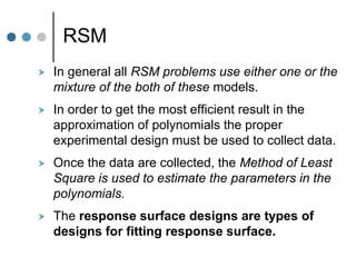
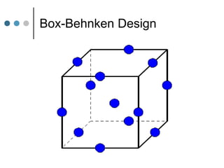
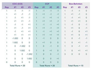
Response Surface Methodology (RSM) uses designed experiments to determine the relationship between several factors and the response. RSM builds a mathematical model to describe this relationship and then uses optimization techniques to find the ideal conditions. Common RSM designs include central composite designs, Box-Behnken designs, and factorial designs. These designs allow modeling of quadratic and interaction effects. The results of RSM experiments are then used to optimize the response through statistical techniques like multiple regression analysis.

1. Response Surface
Methodology (RSM)

2. What is RSM?
RSM can be defines as a statistical method
that uses quantitative data from appropriate
experiments to determine & simultaneously
solve multivarient equations

3. Why RSM?
 Critical factors are known
 Region of interest , where factor levels
influencing product is known
 Factors vary continuously through- out the
experimental range tested
 A mathematical function relates the factors to
the measured response
 The response defined by the function is a
smooth curve

4. illustration
 the growth of a plant is affected by a certain amount
of water x1 and sunshine x2. The plant can grow
under any combination of treatment x1and x2.
 Therefore, water and sunshine can vary
continuously. When treatments are from a
continuous range of values, then a Response
Surface Methodology is useful for developing,
improving, and optimizing the response variable.
 In this case, the plant growth y is the response
variable, and it is a function of water and sunshine. It
can be
 expressed as
 y = f (x1, x2) + e

5. First Order Model
 If the response can be defined by a linear
function of independent variables, then the
approximating function is a first-order model.
 A first-order model with 2 independent
variables can be expressed as
e
x
x
y 


 2
2
1
1
0 



6. Second Order Model
 If there is a curvature in the response surface, then
a higher degree polynomial should be used. The
approximating function with 2 variables is called a
second-order model:
e
x
x
x
x
x
x
y 





 2
1
12
2
22
22
2
11
11
2
2
1
1
0 






7. second degree equation

8. RSM
 In general all RSM problems use either one or the
mixture of the both of these models.
 In order to get the most efficient result in the
approximation of polynomials the proper
experimental design must be used to collect data.
 Once the data are collected, the Method of Least
Square is used to estimate the parameters in the
polynomials.
 The response surface designs are types of
designs for fitting response surface.

9. Objectives
 Therefore, the objective of studying RSM can
be accomplish by
 understanding the topography of the response
surface (local maximum, local minimum, ridge
lines), and
 finding the region where the optimal response
occurs. The goal is to move rapidly and
efficiently along a path to get to a maximum or
a minimum response so that the response is
optimized.

10. Experimental Design
First Degree Models
A. Equiradial designs for 2 factors
B. Equiradial designs for More than 2 factors
– the Simplex Design

11. Experimental Design
Second Degree Models
Spherical Domain
A. Composite Experimental Designs
B. Uniform Shell (Doehlert) Designs
C. Hybrid & Related Desings
D. Equiradial Design for 2 factors – Regular Pentagon
E. Box Behnken Designs

12. Experimental Design
Cubic Shaped Domain
A. Standard Design with 3 levels
- Factorial Designs 3K
- Central Composite Design (α = 1)
- Box Behnken Desing
B. Non Standard Design

13. Equiradial Design for 2 factors

14. The Simplex Design

15. Central Composite Desing
Three distinct sets of experimental runs:
 A factorial design in the factors studied, each
having two levels;
 A set of center points, experimental runs whose
values of each factor are the medians of the
values used in the factorial portion.
 A set of axial points (star point), Each factor is
sequentially placed at ±α and all other factors are
at zero.

16. Central Composite Desing

17. CC Design
Type
Terminol
ogy
Comments
Circumscribe
d
CCC
CCC designs are the original formed CCD. These designs
have circular, spherical, or hyperspherical symmetry and
require 5 levels for each factor. Enlarging an existing
factorial or fractional factorial design with star points can
produce this design.
Inscribed CCI
CCI design uses the factor settings as the star points and
creates a factorial or fractional factorial design within those
limits (in other words, a CCI design is a scaled down CCC
design with each factor level of the CCC design divided by
to generate the CCI design). This design also requires 5
levels of each factor.
Face
Centered
CCF
In this design the star points are at the center of each face
of the factorial space, so = ± 1. This variety requires 3
levels of each factor.

18. Comparison of 3 CC design
 CCC explores the largest process
space and the CCI explores the
smallest process space.
 Both the CCC and CCI are rotatable
designs, but the CCF is not.
 Both the CCC and CCI are require 5
level for each factor while CCF is
require 3 level for each factor.

19. Number of
Factors
Factorial
Portion
Scaled Value for
Relative to ±1
2 22 22/4 = 1.414
3 23 23/4 = 1.682
4 24 24/4 = 2.000
5 25-1 24/4 = 2.000
5 25 25/4 = 2.378
6 26-1 25/4 = 2.378
6 26 26/4 = 2.828
  4
1
2k



20. Design matrix for 2 factor
BLOCK X1 X2
1 -1 -1
1 1 -1
1 -1 1
1 1 1
1 0 0
1 0 0
2 -1.414 0
2 1.414 0
2 0 -1.414
2 0 1.414
2 0 0
2 0 0
Total Runs = 12

21. Design matrix for 3 factor
CCC (CCI)
Rep X1 X2 X3
1 -1 -1 -1
1 +1 -1 -1
1 -1 +1 -1
1 +1 +1 -1
1 -1 -1 +1
1 +1 -1 +1
1 -1 +1 +1
1 +1 +1 +1
1 -1.682 0 0
1 1.682 0 0
1 0 -1.682 0
1 0 1.682 0
1 0 0 -1.682
1 0 0 1.682
6 0 0 0
Total Runs = 20

22. Box-Behnken Design
 The Box-Behnken design is an independent
quadratic design in that it does not contain an
surrounded factorial or fractional factorial
design.
 In this design the treatment combinations are
at the midpoints of edges of the process
space and at the center. These designs are
rotatable (or near rotatable) and require 3
levels of each factor.

23. Box-Behnken Design

24. Box-Behnken Design
Box-Behnken designs are response surface designs, specially made to
require only 3 levels, coded as -1, 0, and +1.
Box-Behnken designs are available for 3 to 10 factors. It is formed by
combining two-level factorial designs with incomplete block designs.
This procedure creates designs with desirable statistical properties but,
most importantly, with only a fraction of the experimental trials
required for a three-level factorial. Because there are only three levels,
the quadratic model was found to be appropriate.
In this design three factors were evaluated, each at three levels, and
experiment design were carried out at all seventeen possible
combinations.

25. CCC (CCI) CCF Box-Behnken
Rep X1 X2 X3 Rep X1 X2 X3 Rep X1 X2 X3
1 -1 -1 -1 1 -1 -1 -1 1 -1 -1 0
1 +1 -1 -1 1 +1 -1 -1 1 +1 -1 0
1 -1 +1 -1 1 -1 +1 -1 1 -1 +1 0
1 +1 +1 -1 1 +1 +1 -1 1 +1 +1 0
1 -1 -1 +1 1 -1 -1 +1 1 -1 0 -1
1 +1 -1 +1 1 +1 -1 +1 1 +1 0 -1
1 -1 +1 +1 1 -1 +1 +1 1 -1 0 +1
1 +1 +1 +1 1 +1 +1 +1 1 +1 0 +1
1 -1.682 0 0 1 -1 0 0 1 0 -1 -1
1 1.682 0 0 1 +1 0 0 1 0 +1 -1
1 0 -1.682 0 1 0 -1 0 1 0 -1 +1
1 0 1.682 0 1 0 +1 0 1 0 +1 +1
1 0 0 -1.682 1 0 0 -1 3 0 0 0
1 0 0 1.682 1 0 0 +1
6 0 0 0 6 0 0 0
Total Runs = 20 Total Runs = 20 Total Runs = 15

26. Case study of
Box Behnken
Experimental Design

27. Batch
Code
Coded value Actual value
X1 X2 X3 X1 X2 X3
B1 -1 1 0 10 15 25
B 2 0 -1 -1 20 5 15
B 3 1 -1 0 30 5 25
B 4 -1 0 -1 10 10 15
B 5 -1 0 1 10 10 35
B 6 0 -1 1 20 5 35
B 7 1 0 1 30 10 35
B 8 -1 -1 0 10 5 25
B 9 0 0 0 20 10 25
B 10 1 1 0 30 15 25
B 11 0 1 -1 20 15 15
B 12 0 1 1 20 15 25
B 13 1 0 -1 30 10 15
B 14 0 0 0 20 10 25
B 15 0 0 0 20 10 25
B 16 0 0 0 20 10 25
B 17 0 0 0 20 10 25
Coded and actual values of Box-Behnken design
The amount of HPMC
K4M (X1),
amount of Carbopol 934P
(X2) and
amount of Sodium
alginate (X3)
were selected as
independent variables.

28. Batch X1
(%)
X2
(%)
X3
(%)
FLTSD
(sec)
TFTSD
(hr)
t50SD
(hr)
nSD
B1 10 15 25 2  1 2.50.35 13.10.03 0.480.02
B2 20 5 15 9  2 10.00.41 12.50.06 0.570.01
B3 30 5 25 4  2 24.00.29 13.30.04 0.520.03
B4 10 10 15 11  2 4.20.32 12.00.07 0.600.02
B5 10 10 35 5  2 5.30.28 11.90.04 0.650.07
B6 20 5 35 3  2 24.00.34 14.80.08 0.520.01
B7 30 10 35 26  4 5.60.35 14.70.05 0.510.01
B8 10 5 25 4  2 8.00.44 12.00.01 0.390.02
B9 20 10 25 3  2 2.50.22 15.80.02 0.440.01
B10 30 15 25 15  3 4.40.14 12.00.04 0.520.03
B11 20 15 15 33  4 3.60.26 12.80.03 0.620.02
B12 20 15 25 15  4 4.90.16 11.10.02 0.470.04
B13 30 10 15 3  1 24.00.36 11.30.05 0.360.06
B14 20 10 25 24  3 4.80.18 10.50.04 0.500.01
B15 20 10 25 10  2 6.80.45 15.00.07 0.480.04
B16 20 10 25 6  2 7.00.0.3
6
13.20.06 0.700.03
B17 20 10 25 12  2 4.20.26 13.20.03 0.450.02

29. 29
Multiple Regression
It is an extension of linear regression in
which we wish to relate a response, Y
dependent variables to more than one
independent variable
• Linear Regression
Y = A+ BY
• Multiple Regression
Y = bo + b1X1 + b2X2+….
X1, X2, …. Represent factors which influence the
response

30. 30
Y = bo + b1X1 + b2X2 + b3X3…
Y is response i.e. dissolution time
Xi is independent variable
bo is the intercept
bi is regression coefficient for the ith
independent variable
X1, X2, X3.. Are the levels of variables

31. The Polynomial equation generated by this experimental design is
described as:
Yi = b0 + b1x1 +b2x2 + b3x3 + b12x1x2 + b13 x1x3 + b23x2x3 +
b11x12 +b22x22 + b33x32
Where Yi is the dependent variable
b0 is the intercept; bi, bij and bijk represents the regression
coefficients
Xi represents the level of independent variables which were
selected from the preliminary experiments.