Unit iii Correlation and Regression

1. Unit-III
Describing Relationships

2. Correlation
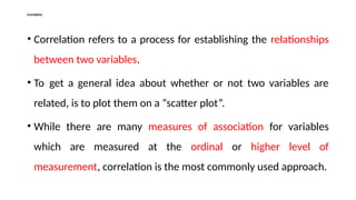
• Correlation refers to a process for establishing the relationships
between two variables.
• To get a general idea about whether or not two variables are
related, is to plot them on a “scatter plot”.
• While there are many measures of association for variables
which are measured at the ordinal or higher level of
measurement, correlation is the most commonly used approach.

3. Types of Correlation
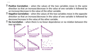
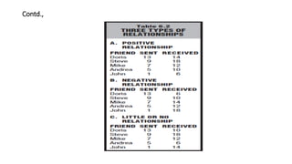
 Positive Correlation – when the values of the two variables move in the same
direction so that an increase/decrease in the value of one variable is followed by
an increase/decrease in the value of the other variable.
 Negative Correlation – when the values of the two variables move in the opposite
direction so that an increase/decrease in the value of one variable is followed by
decrease/increase in the value of the other variable.
 No Correlation – when there is no linear dependence or no relation between the
two variables.

4. Contd.,

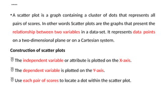
5. Scatterplots
• A scatter plot is a graph containing a cluster of dots that represents all
pairs of scores. In other words Scatter plots are the graphs that present the
relationship between two variables in a data-set. It represents data points
on a two-dimensional plane or on a Cartesian system.
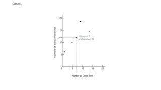
Construction of scatter plots
 The independent variable or attribute is plotted on the X-axis.
 The dependent variable is plotted on the Y-axis.
 Use each pair of scores to locate a dot within the scatter plot.

6. Contd.,

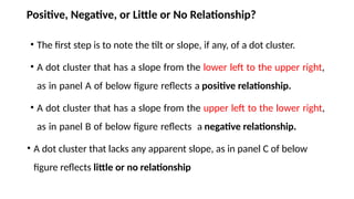
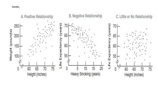
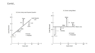
7. Positive, Negative, or Little or No Relationship?
• The first step is to note the tilt or slope, if any, of a dot cluster.
• A dot cluster that has a slope from the lower left to the upper right,
as in panel A of below figure reflects a positive relationship.
• A dot cluster that has a slope from the upper left to the lower right,
as in panel B of below figure reflects a negative relationship.
• A dot cluster that lacks any apparent slope, as in panel C of below
figure reflects little or no relationship

8. Contd.,

9. Perfect Relationship
• A dot cluster that equals (rather than merely approximates) a straight
line reflects a perfect relationship between two variables.
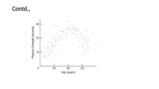
Curvilinear Relationship
• A dot cluster approximates a straight line and, therefore, reflects a
linear relationship. But this is not always the case. Sometimes a dot
cluster approximates a bent or curved line, as in below figure, and
therefore reflects a curvilinear relationship.

10. Contd.,

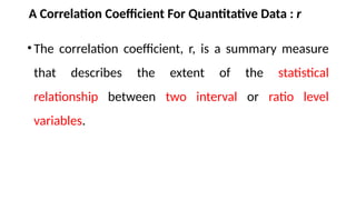
11. A Correlation Coefficient For Quantitative Data : r
•The correlation coefficient, r, is a summary measure
that describes the extent of the statistical
relationship between two interval or ratio level
variables.

12. Properties of r
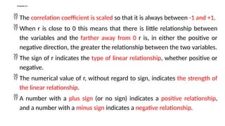
 The correlation coefficient is scaled so that it is always between -1 and +1.
 When r is close to 0 this means that there is little relationship between
the variables and the farther away from 0 r is, in either the positive or
negative direction, the greater the relationship between the two variables.
 The sign of r indicates the type of linear relationship, whether positive or
negative.
 The numerical value of r, without regard to sign, indicates the strength of
the linear relationship.
 A number with a plus sign (or no sign) indicates a positive relationship,
and a number with a minus sign indicates a negative relationship.

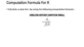
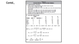
13. Computation Formula For R
• Calculate a value for r by using the following computation formula:

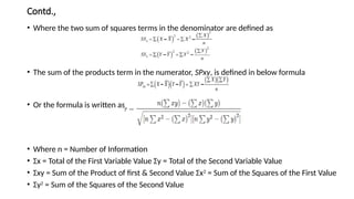
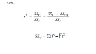
14. Contd.,
• Where the two sum of squares terms in the denominator are defined as
• The sum of the products term in the numerator, SPxy, is defined in below formula
• Or the formula is written as
• Where n = Number of Information
• Σx = Total of the First Variable Value Σy = Total of the Second Variable Value
• Σxy = Sum of the Product of first & Second Value Σx2
= Sum of the Squares of the First Value
• Σy2
= Sum of the Squares of the Second Value

15. Contd.,

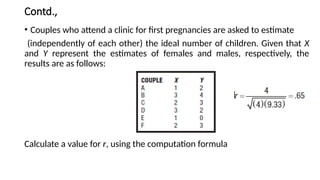
16. Contd.,
• Couples who attend a clinic for first pregnancies are asked to estimate
(independently of each other) the ideal number of children. Given that X
and Y represent the estimates of females and males, respectively, the
results are as follows:
Calculate a value for r, using the computation formula

17. Regression
• A regression is a statistical technique that relates a dependent variable to one
or more independent (explanatory) variables.
• A regression model is able to show whether changes observed in the
dependent variable are associated with changes in one or more of the
explanatory variables.
• Regression captures the correlation between variables observed in a data set,
and quantifies whether those correlations are statistically significant or not.
https://www.youtube.com/watch?v=-JTKf-a1JpU
https://www.youtube.com/watch?v=i3IadpjctWg

18. A Regression Line
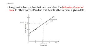
• A regression line is a line that best describes the behavior of a set of
data. In other words, it’s a line that best fits the trend of a given data.

19. Contd.,
• The purpose of the line is to describe the interrelation of a dependent
variable (Y variable) with one or many independent variables (X variable).
• By using the equation obtained from the regression line an analyst can
forecast future behaviors of the dependent variable by inputting different
values for the independent ones.
• https://www.w3schools.com/python/python_ml_linear_regression.asp
• https://www.geeksforgeeks.org/machine-learning/ml-multiple-linear-
regression-using-python/

20. Types of regression
• The two basic types of regression are
• Simple linear regression
• Simple linear regression uses one independent variable to explain or
predict the outcome of the dependent variable Y
• Multiple linear regression
• Multiple linear regressions use two or more independent variables to
predict the outcome

21. Predictive Errors
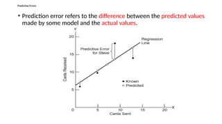
• Prediction error refers to the difference between the predicted values
made by some model and the actual values.

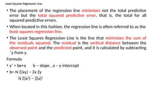
22. Least Squares Regression Line
• The placement of the regression line minimizes not the total predictive
error but the total squared predictive error, that is, the total for all
squared predictive errors.
• When located in this fashion, the regression line is often referred to as the
least squares regression line.
• The Least Squares Regression Line is the line that minimizes the sum of
the residuals squared. The residual is the vertical distance between the
observed point and the predicted point, and it is calculated by subtracting
ˆy from y.
Formula
• y’ = bx+a b – slope , a – y intercept
• b= N Σ(xy) − Σx Σy
N Σ(x2
) − (Σx)2

23. Contd.,
• b = Σy − m Σx
N
X Y
2 4
3 5
5 7
7 10
9 15

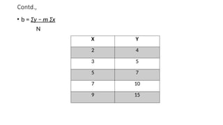
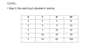
24. Contd.,
• Step 1: For each (x,y) calculate x2
and xy:
X Y X2
XY
2 4 4 8
3 5 9 15
5 7 25 35
7 10 49 70
9 15 81 135

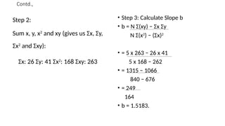
25. Contd.,
Step 2:
Sum x, y, x2
and xy (gives us Σx, Σy,
Σx2
and Σxy):
Σx: 26 Σy: 41 Σx2
: 168 Σxy: 263
• Step 3: Calculate Slope b
• b = N Σ(xy) − Σx Σy
N Σ(x2
) − (Σx)2
• = 5 x 263 − 26 x 41
5 x 168 − 262
• = 1315 − 1066
840 − 676
• = 249
164
• b = 1.5183.

26. Contd.,
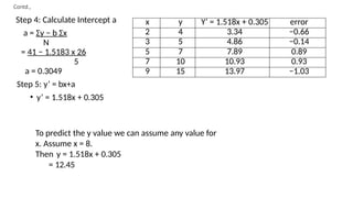
Step 4: Calculate Intercept a
a = Σy − b Σx
N
= 41 − 1.5183 x 26
5
a = 0.3049
Step 5: y’ = bx+a
• y’ = 1.518x + 0.305
x y Y’ = 1.518x + 0.305 error
2 4 3.34 −0.66
3 5 4.86 −0.14
5 7 7.89 0.89
7 10 10.93 0.93
9 15 13.97 −1.03
To predict the y value we can assume any value for
x. Assume x = 8.
Then y = 1.518x + 0.305
= 12.45

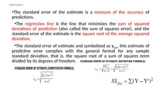
27. Standard Error Of Estimate ,s y | x
•The standard error of the estimate is a measure of the accuracy of
predictions.
•The regression line is the line that minimizes the sum of squared
deviations of prediction (also called the sum of squares error), and the
standard error of the estimate is the square root of the average squared
deviation.
•The standard error of estimate and symbolized as sy|x, this estimate of
predictive error complies with the general format for any sample
standard deviation, that is, the square root of a sum of squares term
divided by its degrees of freedom.

28. Contd.,

29. Contd.,
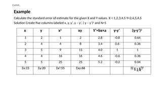
Example
Calculate the standard error of estimate for the given X and Y values. X = 1,2,3,4,5 Y=2,4,5,4,5
Solution Create five columns labeled x, y, y’, y – y’, ( y – y’)2
and N=5
x y x2
xy Y’=bx+a y-y’ (y-y’)2
1 2 1 2 2.8 -0.8 0.64
2 4 4 8 3.4 0.6 0.36
3 5 9 15 4.0 1 1
4 4 16 16 4.6 -0.6 0.36
5 5 25 25 5.2 -0.2 0.04
Σx:15 Σy:20 Σx2
:55 Σxy:66 Σ( y – y’)2
= 2.4

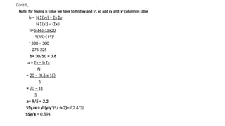
30. Contd.,
Note: for finding b value we have to find xy and x2
, so add xy and x2
column in table
b = N Σ(xy) − Σx Σy
N Σ(x2
) − (Σx)2
b=5(66)-15x20
5(55)-(15)2
=
330 – 300
275-225
b= 30/50 = 0.6
a = Σy − b Σx
N
= 20 – (0.6 x 15)
5
= 20 – 11
5
a= 9/5 = 2.2
SSy/x = √((y-y’)2
/ n-2)=√(2.4/3)
SSy/x = 0.894

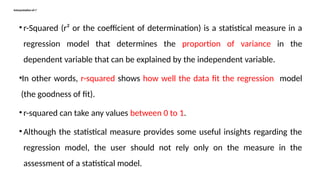
31. Interpretation of r2
• r-Squared (r² or the coefficient of determination) is a statistical measure in a
regression model that determines the proportion of variance in the
dependent variable that can be explained by the independent variable.
•In other words, r-squared shows how well the data fit the regression model
(the goodness of fit).
• r-squared can take any values between 0 to 1.
• Although the statistical measure provides some useful insights regarding the
regression model, the user should not rely only on the measure in the
assessment of a statistical model.

32. Contd.,
• In addition, it does not indicate the correctness of the regression
model. Therefore, the user should always draw conclusions about the
model by analyzing r-squared together with the other variables in a
statistical model.
• The most common interpretation of r-squared is how well the
regression model explains observed data.

33. Contd.,

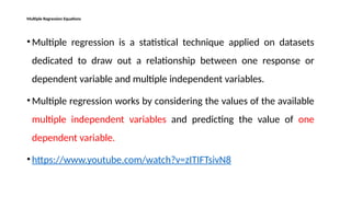
34. Multiple Regression Equations
• Multiple regression is a statistical technique applied on datasets
dedicated to draw out a relationship between one response or
dependent variable and multiple independent variables.
• Multiple regression works by considering the values of the available
multiple independent variables and predicting the value of one
dependent variable.
• https://www.youtube.com/watch?v=zITIFTsivN8

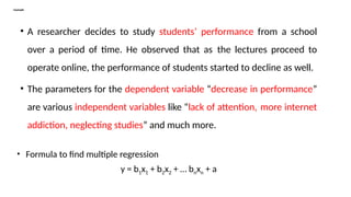
35. Example
• A researcher decides to study students’ performance from a school
over a period of time. He observed that as the lectures proceed to
operate online, the performance of students started to decline as well.
• The parameters for the dependent variable “decrease in performance”
are various independent variables like “lack of attention, more internet
addiction, neglecting studies” and much more.
• Formula to find multiple regression
y = b1x1 + b2x2 + … bnxn + a

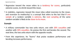
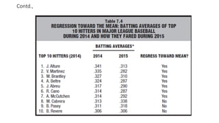
36. Regression Toward The Mean
• Regression toward the mean refers to a tendency for scores, particularly
extreme scores, to shrink toward the mean.
• In statistics, regression toward the mean (also called reversion to the mean,
and reversion to mediocrity) is a concept that refers to the fact that if one
sample of a random variable is extreme, the next sampling of the same
random variable is likely to be closer to its mean.
Example
• A military commander has two units return, one with 20% casualties and
another with 50% casualties. He praises the first and berates the second. The
next time, the two units return with the opposite results.
• From this experience, he “learns” that praise weakens performance and
berating increases performance.

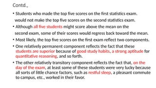
37. Contd.,
• Students who made the top five scores on the first statistics exam.
would not make the top five scores on the second statistics exam.
• Although all five students might score above the mean on the
second exam, some of their scores would regress back toward the mean.
• Most likely, the top five scores on the first exam reflect two components.
• One relatively permanent component reflects the fact that these
students are superior because of good study habits, a strong aptitude for
quantitative reasoning, and so forth.
• The other relatively transitory component reflects the fact that, on the
day of the exam, at least some of these students were very lucky because
all sorts of little chance factors, such as restful sleep, a pleasant commute
to campus, etc., worked in their favor.

38. Contd.,
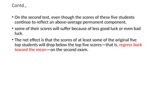
• On the second test, even though the scores of these five students
continue to reflect an above-average permanent component,
• some of their scores will suffer because of less good luck or even bad
luck.
• The net effect is that the scores of at least some of the original five
top students will drop below the top five scores—that is, regress back
toward the mean—on the second exam.

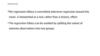
39. The Regression Fallacy
•The regression fallacy is committed whenever regression toward the
mean is interpreted as a real, rather than a chance, effect.
• The regression fallacy can be avoided by splitting the subset of
extreme observations into two groups.

40. Contd.,

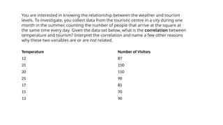
41. You are interested in knowing the relationship between the weather and tourism
levels. To investigate, you collect data from the touristic centre in a city during one
month in the summer, counting the number of people that arrive at the square at
the same time every day. Given the data set below, what is the correlation between
temperature and tourism? Interpret the correlation and name a few other reasons
why these two variables are or are not related.
Temperature Number of Visitors
12 87
21 150
20 110
25 90
17 85
15 70
13 90

42. • Page no:144