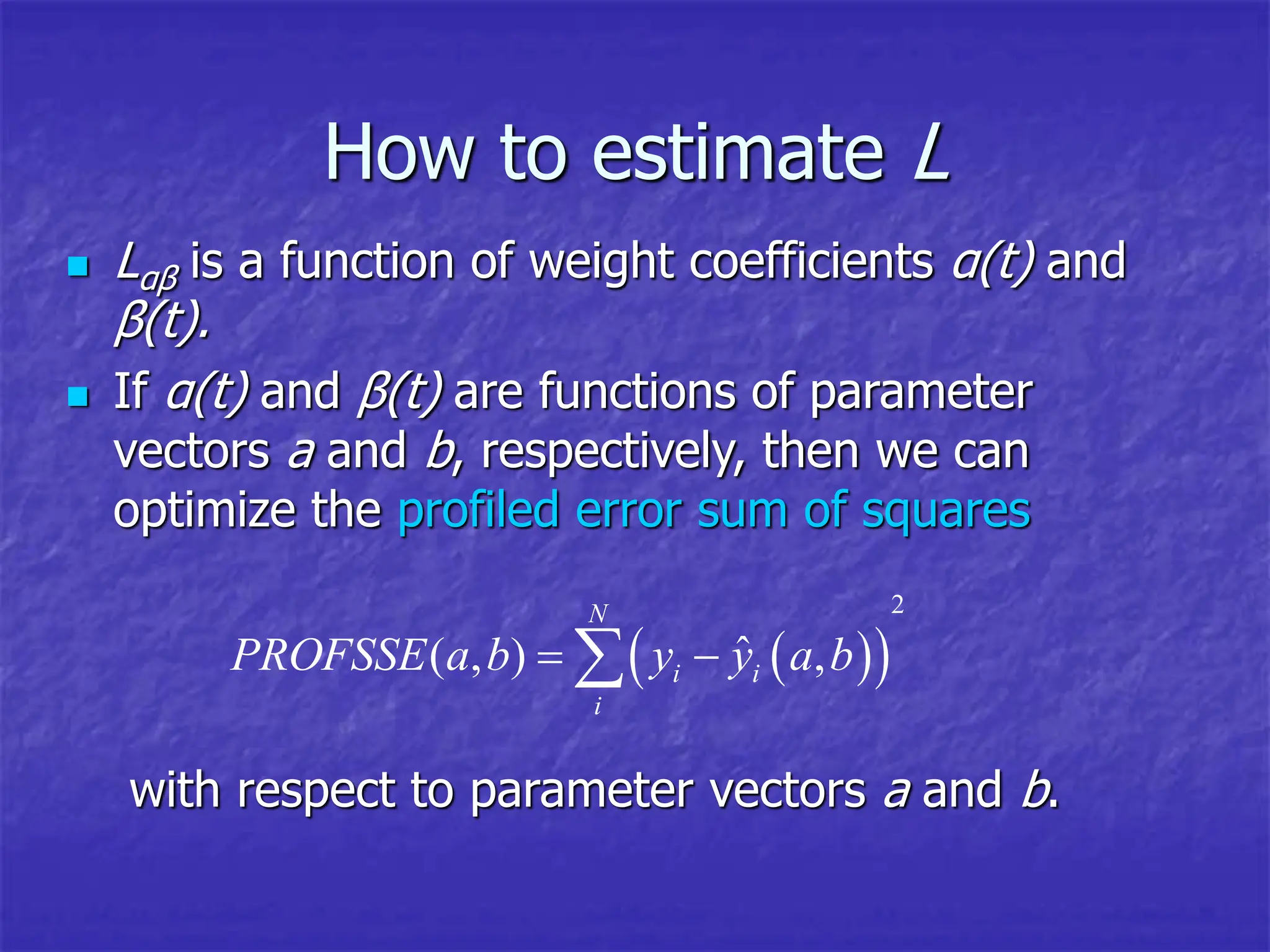
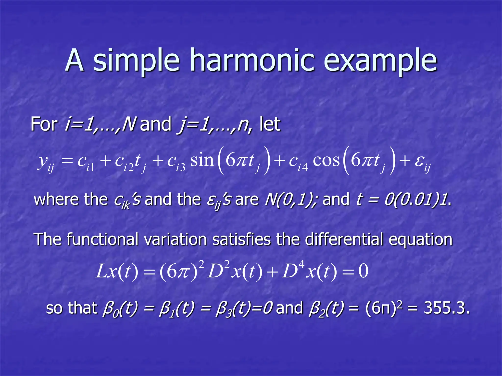
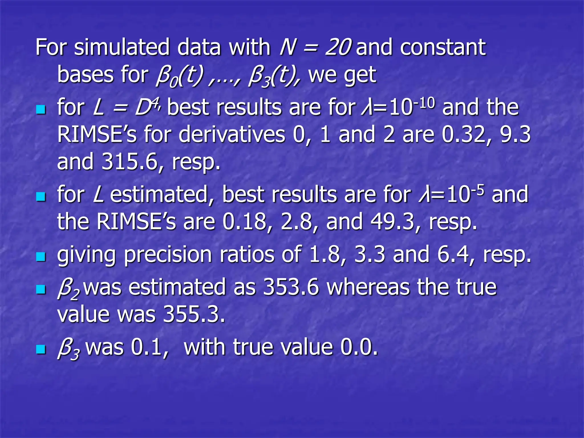
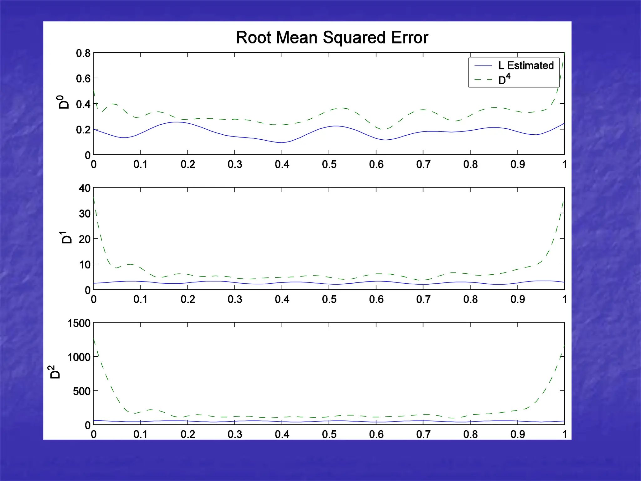
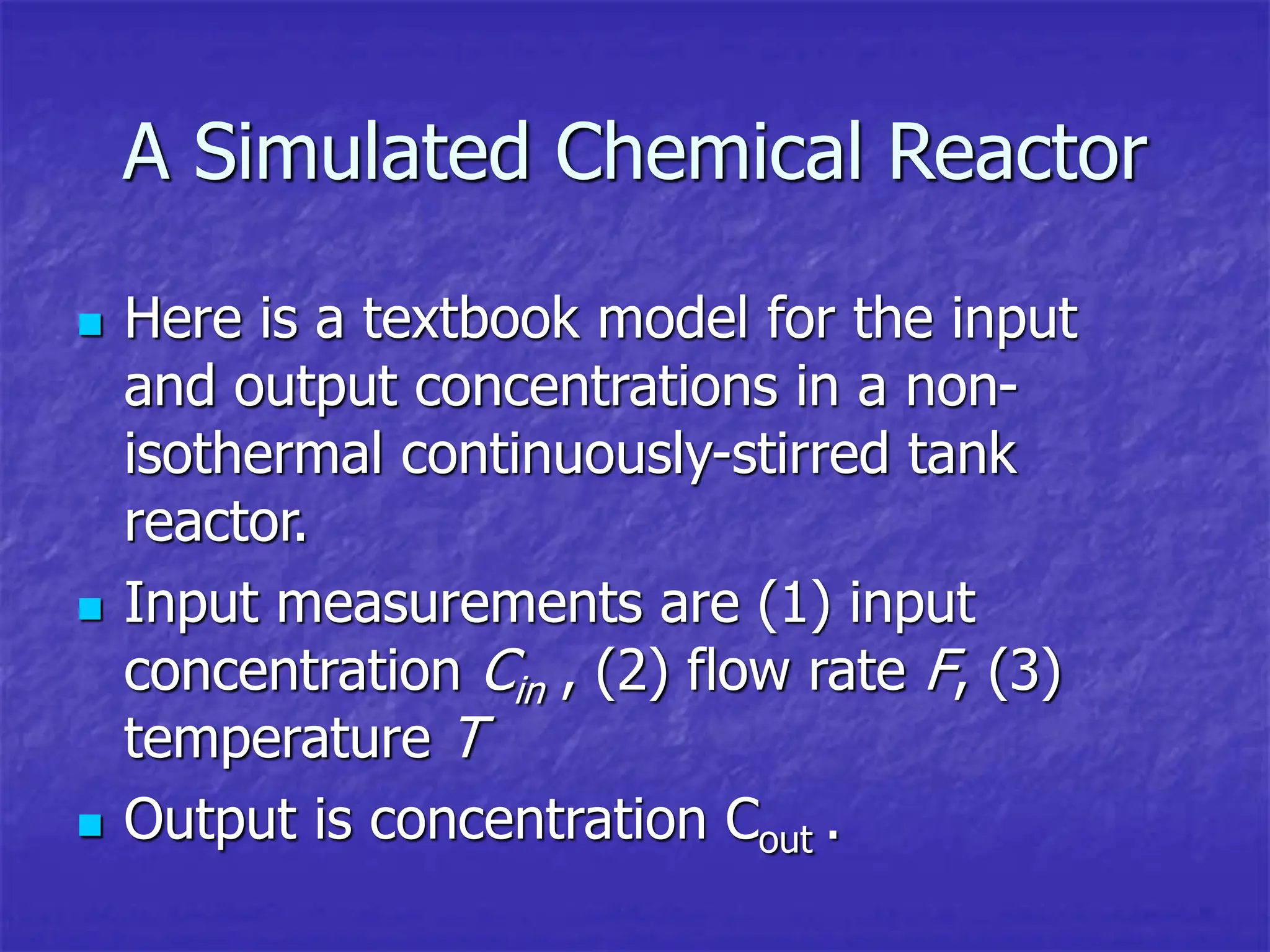
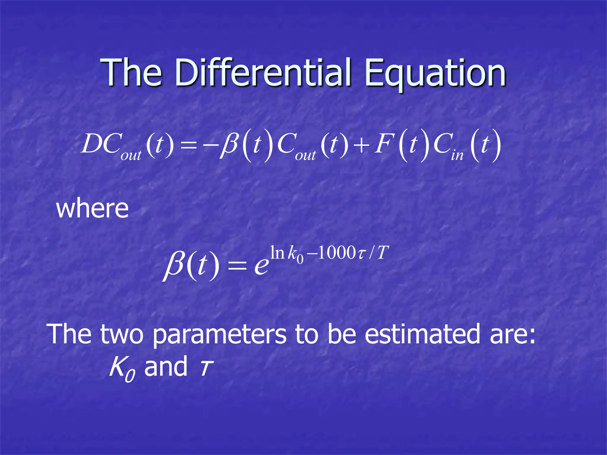
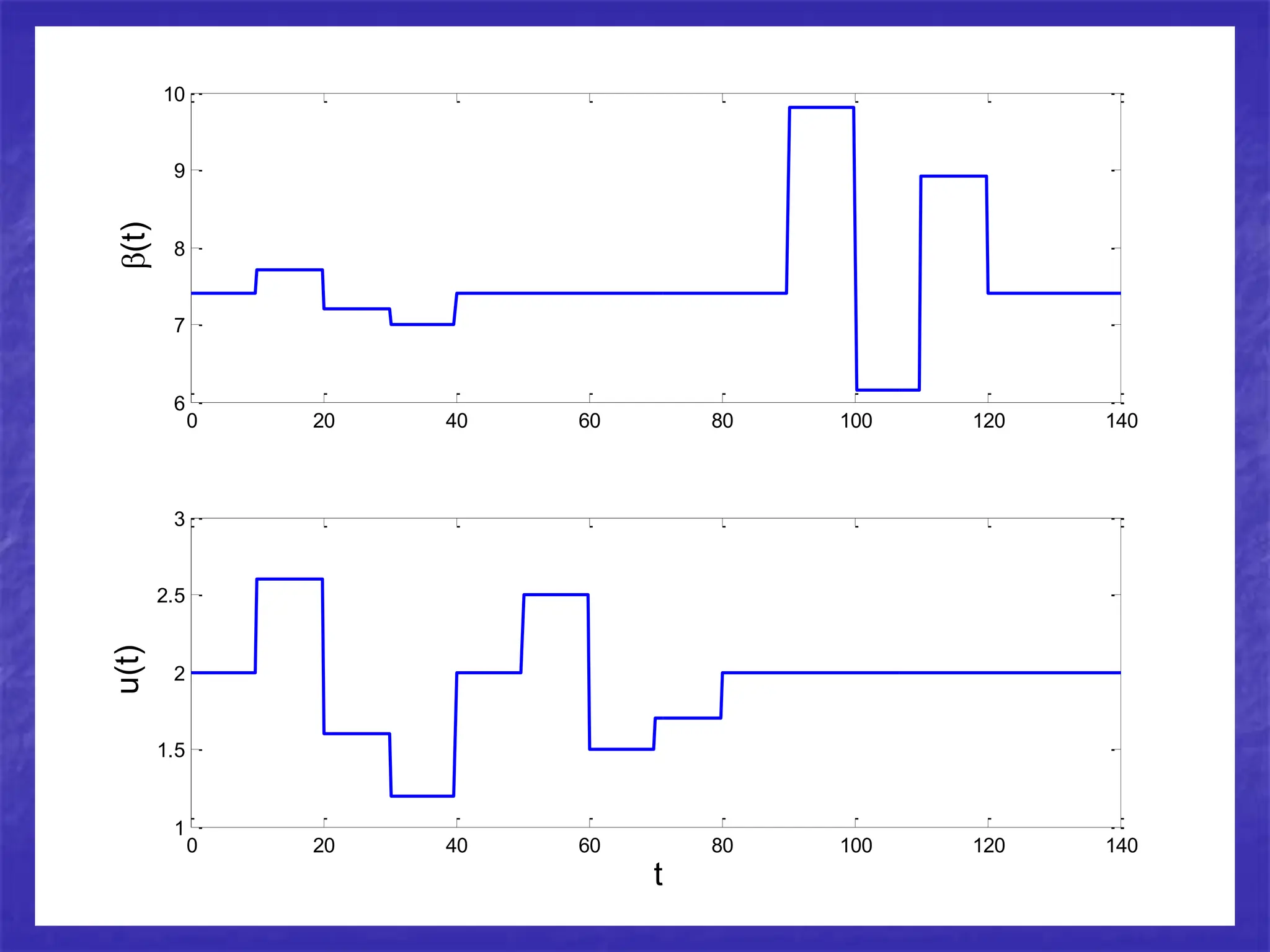
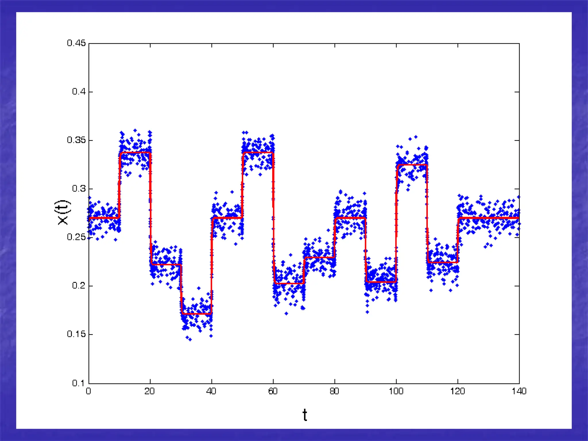
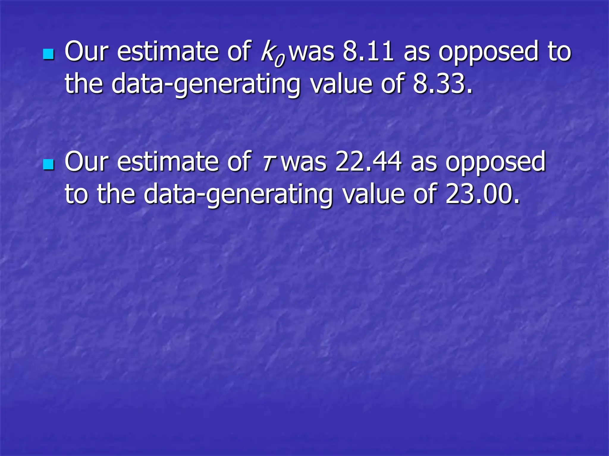
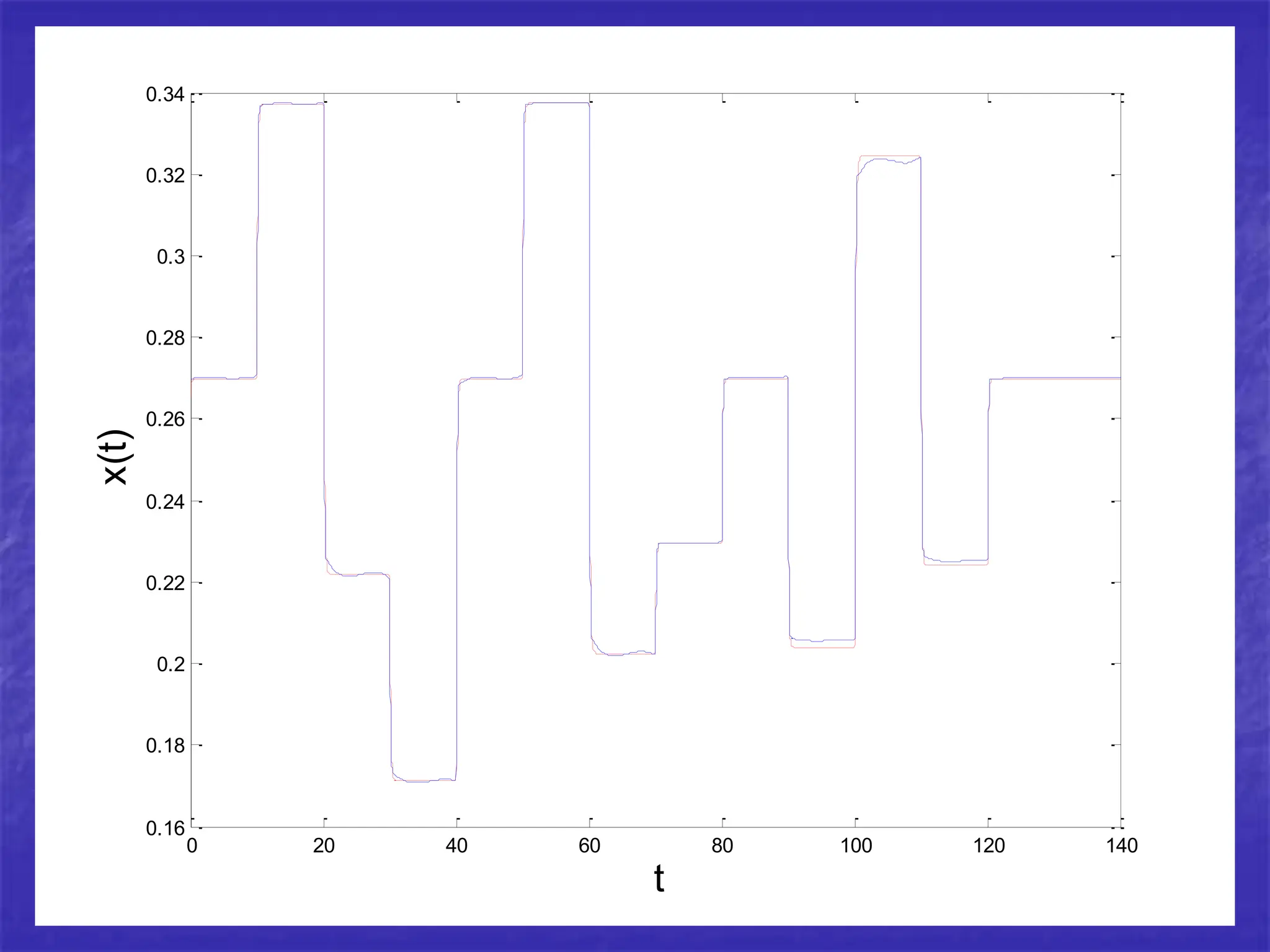
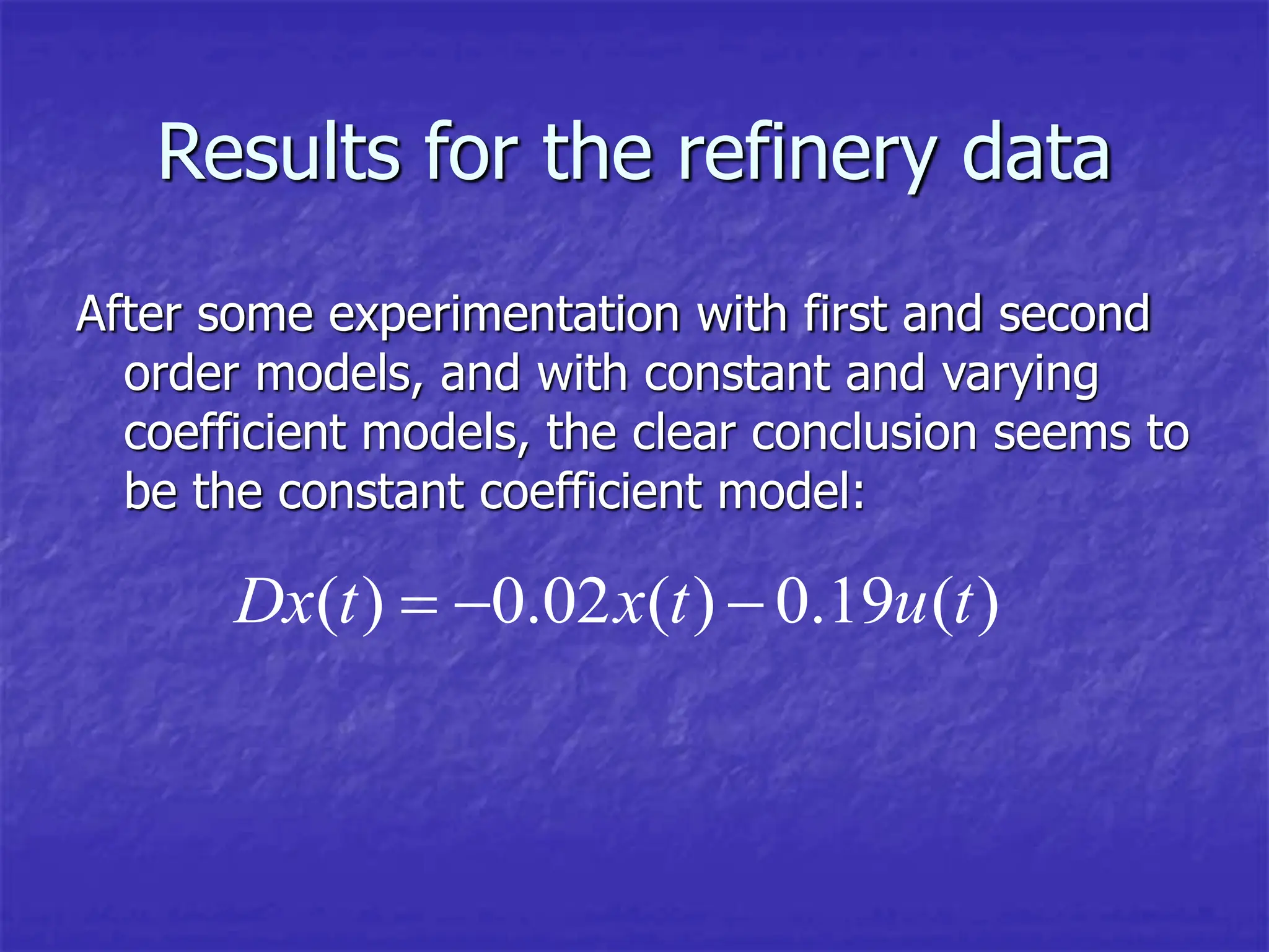
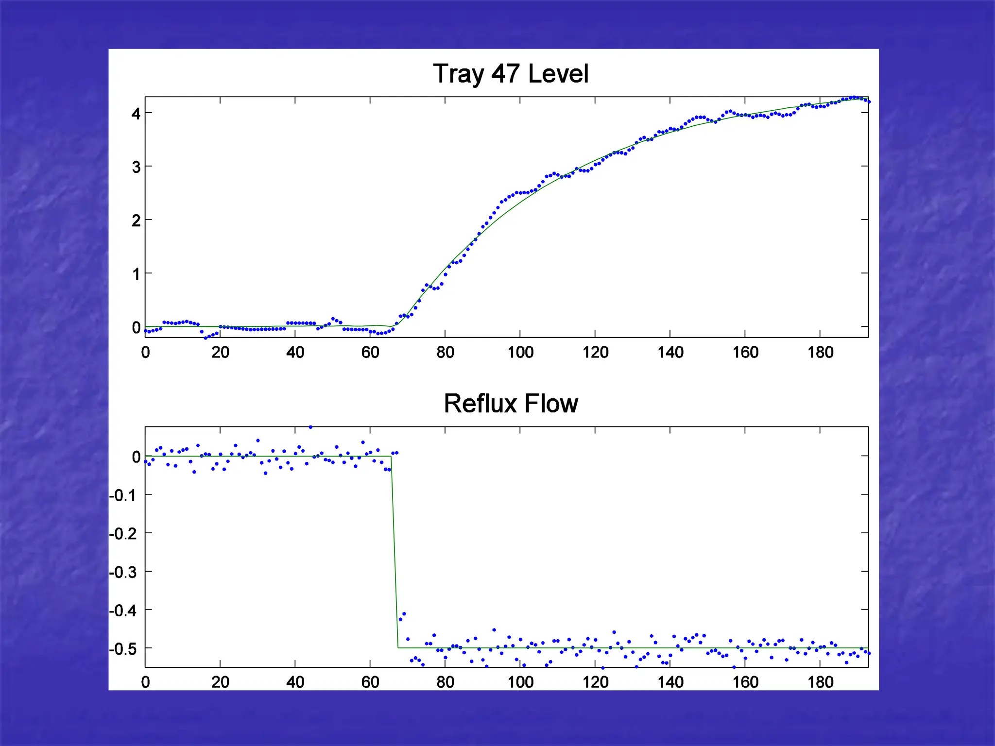
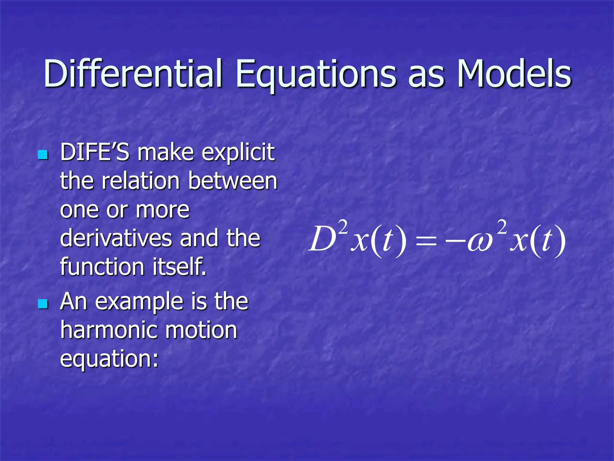
Differential equations can be powerful tools for modeling data. New methods allow estimating differential equations directly from data. As an example, the author estimates a differential equation model from simulated data from a chemical reactor. The estimated parameters are close to the true values, demonstrating the method works well on simulated data.

1. From Data to Differential
Equations
Jim Ramsay
McGill University
( ) [ ( ), ]
Dx t f x t t


2. The themes
 Differential equations are powerful tools
for modeling data.
 There are new methods for estimating
differential equations directly from data.
 Some examples are offered, drawn from
chemical engineering and medicine.

3. Differential Equations as Models
 DIFE’S make explicit
the relation between
one or more
derivatives and the
function itself.
 An example is the
harmonic motion
equation:
2 2
( ) ( )
D x t x t

 

4. Why Differential Equations?
 The behavior of a derivative is often of more
interest than the function itself, especially over
short and medium time periods.
 What often counts is how rapidly a system
responds rather than its level of response.
 Velocity and acceleration can reflect energy
exchange within a system.
 Recall equations like f = ma and e = mc2.

5.  Natural scientists often provide theory to
biologists and engineers in the form of
DIFE’s.
 Many fields such as pharmacokinetics and
industrial process control routinely use
DIFE’s as models, especially for
input/output systems.
 DIFE’s are especially useful when feedback
systems must be developed to control the
behavior of systems.

6.  The solution to an mth order linear DIFE is
an m-dimensional function space, and thus
the equation can model variation over
replications as well as average behavior.
 Systems of DIFE’s are important models
for processes mutually influencing each
other, such as treatments and symptoms,
predator and prey, and etc.

7.  DIFE’s require that derivatives are smooth,
since they link the behavior of derivatives
to that of the function itself.
 Even simple nonlinear differential
equations can imply function
characteristics that would be impossible to
model in any other way.

8. The Rössler Equations
This nearly linear system exhibits chaotic behavior
that would be virtually impossible to model
without using a DIFE:
( ) ( ) ( )
( ) ( ) ( )
( ) ( ( ) ) ( )
Dx t y t z t
Dy t x t ay t
Dz t b x t c z t
  
 
  

9. Stochastic DIFE’s
We can introduce stochastic elements into
DIFE’s in many ways:
 Random coefficient functions.
 Random forcing functions.
 Random initial, boundary, and other
constraints.
 Stochastic time.

10. Differential equations and time
scales
 DIFE’s are important where there are
events at different time scales.
 The order of the equation plus one
corresponds to the number of time scales.
 A first-order equation can model events on
two time scales: long-term, modeled by
x(t), and short-term, modeled by Dx(t).

11. Handwriting has four time scales
 Average spatial position needs only x(t), time
scale is many seconds.
 Overall left-to-right trend requires Dx(t) , with a
time scale a second or less.
 Cusps, loops, strokes require D2x(t) , with a time
scale of 100 msec or so.
 Transient effects such from pen contacting paper
require D3x(t) with a scale of 10 msec.

12. If we can model data on functions or
functional input/output systems, we will
have a modeling tool that greatly extends
the power and scope of existing
nonparametric curve-fitting techniques.
These models will be dynamic in the sense of
also modeling the rate of change in the
system.
We may also get better estimates of
functional parameters and their derivatives.

13. A simple input/output system
 We begin by looking at a first order DIFE
for a single output function x(t) and a
single input function u(t). (SISO)
 But our goal is the linking of multiple
inputs to multiple outputs (MIMO) by
linear or nonlinear systems of arbitrary
order m.

14. ( ) ( ) ( ) ( ) ( )
Dx t t x t t u t
 
  
•u(t) is often called the forcing function.
•α(t) and β(t) are the coefficient functions
that define the DIFE.
•The system is linear in these coefficient
functions, and in the input u(t) and output
x(t).

15. In this simple case, an analytic solution is
possible:
 
0
( ) ( )[ (0) [ ( )/ ( )] ]
t
x t h t x s u s h s ds

  
However, in most situations involving
DIFE’s it is necessary to use numerical
methods to find the solution.
where
0
( )
( )
t
s ds
h t e




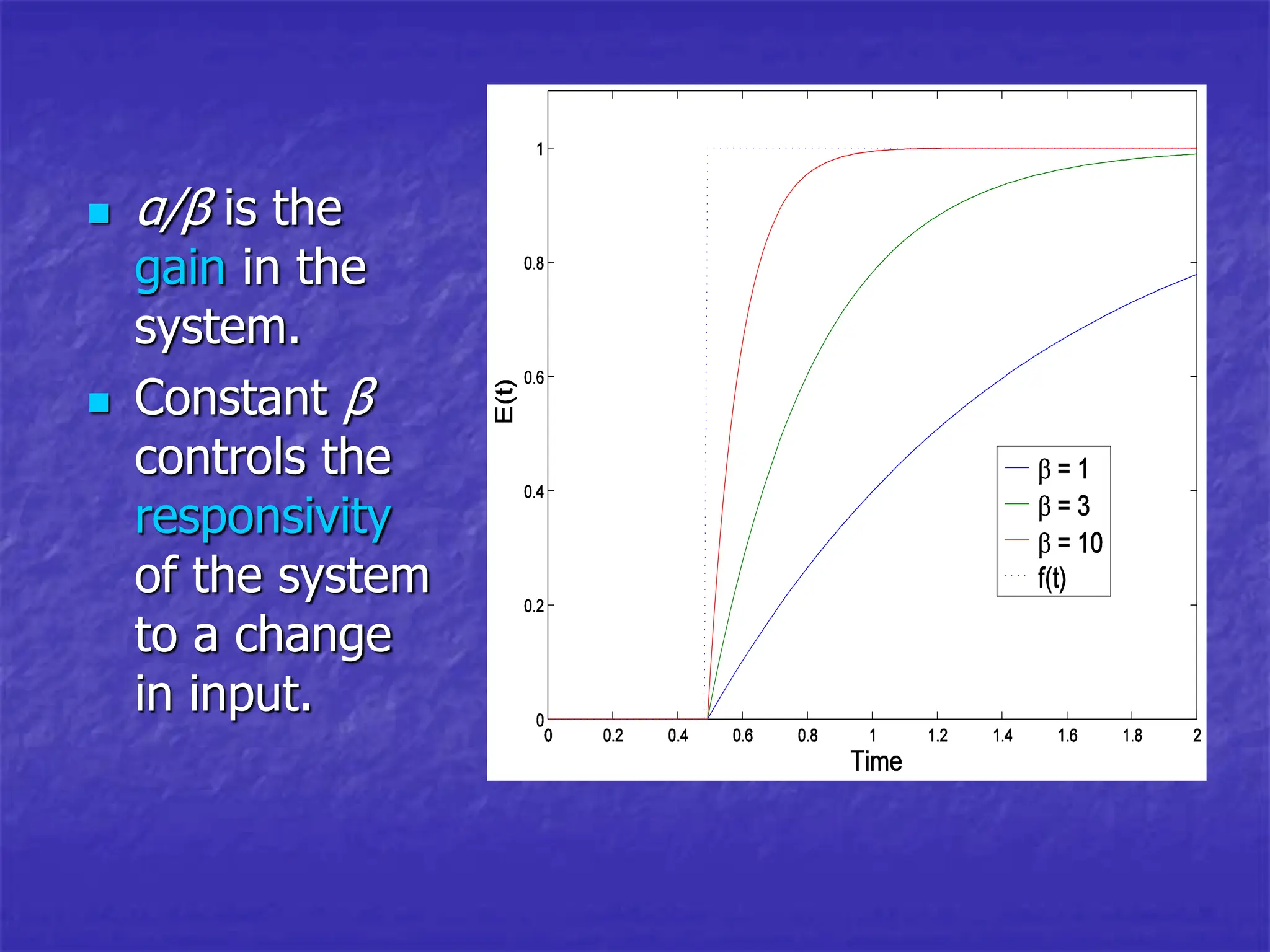
16. A constant coefficient example
We can see more clearly what happens
when
 Coefficients α and β are constants,
 u(t) is a function stepping from 0 to 1
at time t1:
1
( )
1
( ) [1 ],
t t
x t e t t



 
  

17.  α/β is the
gain in the
system.
 Constant β
controls the
responsivity
of the system
to a change
in input.

18. How can we estimate a
DIFE from noisy data?

19. The DIFE as a linear differential
operator
We can express the first order DIFE as a linear
differential operator:
( ) ( ) ( ) ( ) ( ) ( ) 0
L x t t x t Dx t t u t
  
   
More generally, dropping “(t)”,
1
0 1
m K
j m
j k k
j k
L x D x D x u
  

 
  
 

20. Smoothing data with the operator L
If we know the differential equation, then the
operator Lαβ can define a data smoother. The
penalized least squares fitting criterion is:
 
2
2
1
( ) ( )
N
i i
i
PENSSE y x t L x t dt



 
    
 
The larger λ is, the more the fitting function x(t)
is forced to be a solution of the differential equation
Lαβx(t) = 0.

21. The smooth values
If x(t) is expanded in terms of a set K basis
functions φk(t), and if N by K matrix Z contains
the values of these functions at time points ti,
then the vector fitting the data is
     
        
1
, [ ' , ] '[ , ]
, ', ,
y Z Z Z R Z y s
R L L s L u
  
       
      

  
 
 

22. How to estimate L
 Lαβ is a function of weight coefficients α(t) and
β(t).
 If α(t) and β(t) are functions of parameter
vectors a and b, respectively, then we can
optimize the profiled error sum of squares
 
 
2
ˆ
( , ) ,
N
i i
i
PROFSSE a b y y a b
 

with respect to parameter vectors a and b.

23. Adding constraints
It is a simple matter to:
 Constrain some coefficient functions to be
zero or a constant.
 Force others to be smooth, employing
specific linear differential operators to
smooth them towards specific target
spaces.

24. And more …
This approach is easily generalizable to:
 DIFE’s and differential operators of any
order.
 Multiple inputs uj(t) and outputs xi(t).
 Replicated functional data.
 Nonlinear DIFE’s and operators.

25. What about choosing λ?
 Choosing the smoothing parameter λ is always a
delicate matter.
 The right value of λ will be rather large if the
data can be well-modeled by a low-order DIFE,
but not so large as to fail to smooth
observational noise and small additional
functional variation.
 Generalized cross-validation seems to work.

26. Some Simulations
 Let’s see how well this method works
where we know what we’re estimating.

27. A simple harmonic example
For i=1,…,N and j=1,…,n, let
   
1 2 3 4
sin 6 cos 6
ij i i j i j i j ij
y c c t c t c t
  
    
where the cik’s and the εij’s are N(0,1); and t = 0(0.01)1.
The functional variation satisfies the differential equation
2 2 4
( ) (6 ) ( ) ( ) 0
Lx t D x t D x t

  
so that β0(t) = β1(t) = β3(t)=0 and β2(t) = (6π)2 = 355.3.

29. For simulated data with N = 20 and constant
bases for β0(t) ,…, β3(t), we get
 for L = D4, best results are for λ=10-10 and the
RIMSE’s for derivatives 0, 1 and 2 are 0.32, 9.3
and 315.6, resp.
 for L estimated, best results are for λ=10-5 and
the RIMSE’s are 0.18, 2.8, and 49.3, resp.
 giving precision ratios of 1.8, 3.3 and 6.4, resp.
 β2 was estimated as 353.6 whereas the true
value was 355.3.
 β3 was 0.1, with true value 0.0.

31.  In addition to better curve estimates and
much better derivative estimates, note
that the derivative RMSE’s do not go wild
at the end points.
 This is because the DIFE ties the
derivatives to the function values, and the
function values are tamed by the data.

32. A decaying harmonic example
A second order equation defining harmonic
behavior with decay, forced by a step
function:
 β0 = 4.04, β1 = 0.4, α = -2.0.
 u(t) = 0, t < 2π, u(t) = 1, t ≥ 2π.
 Noise with std. dev. 0.2 added to 100
randomly generated solution functions.

33. 0 2 4 6 8 10 12
-1.5
-1
-0.5
0
0.5
1
1.5
2
t
data
x(t)
u(t)

34. Parameter True Value Mean
Estimate
Std. Error
β0 4.040 4.041 0.073
β1 0.400 0.397 0.048
α -2.000 -1.998 0.088
Results from 100 samples using minimum
generalized cross-validation to choose λ:

35. Monotone smoothing
 Some constrained
functions can be
expressed as DIFE’s.
 A smooth strictly
monotone function
can be expressed as
the second order
DIFE
2
( ) ( ) ( )
D x t t Dx t



36.  We can monotonically smooth data by
estimating the second order DIFE directly.
 We constrain β0(t) = 0, and give β1(t) enough
flexibility to smooth the data.
 In the following artificial example, the
smoothing parameter was chosen by
generalized cross-validation. β1(t) was expanded
in terms of 13 B-splines.

37. 0 0.1 0.2 0.3 0.4 0.5 0.6 0.7 0.8 0.9 1
-0.5
0
0.5
1
1.5
2
2.5
3
3.5
4
t
x(t)
Data
Estimate
True

38. 0 0.1 0.2 0.3 0.4 0.5 0.6 0.7 0.8 0.9 1
0
2
4
6
8
10
12
t
Dx(t)
Data
Estimate
True

39. A Simulated Chemical Reactor
 Here is a textbook model for the input
and output concentrations in a non-
isothermal continuously-stirred tank
reactor.
 Input measurements are (1) input
concentration Cin , (2) flow rate F, (3)
temperature T
 Output is concentration Cout .

40. The Differential Equation
     
( ) ( )
out out in
DC t t C t F t C t

  
0
ln 1000 /
( ) k T
t e 
 

The two parameters to be estimated are:
K0 and τ
where

41. Process control experiments
 Engineers studying systems like these like
to carry out experiments in which inputs
are stepped up or down at random times.
 They infer the dynamics of the process
from the impacts of these steps on the
output(s).

42. 0 20 40 60 80 100 120 140
6
7
8
9
10
(t)
0 20 40 60 80 100 120 140
1
1.5
2
2.5
3
t
u(t)

43.  We solved this differential equation for
known values of the two unknown
parameters,
 and then added zero mean Gaussian error
with a standard deviation of 0.01.

45.  Our estimate of k0 was 8.11 as opposed to
the data-generating value of 8.33.
 Our estimate of τ was 22.44 as opposed
to the data-generating value of 23.00.

46. 0 20 40 60 80 100 120 140
0.16
0.18
0.2
0.22
0.24
0.26
0.28
0.3
0.32
0.34
t
x(t)

47. A Real-Data Example

48. Flow in an oil refinery distillation
column
 The single input is “reflux flow” and the
output is “tray 47” level.
 There were 194 sampling points.
 30 B-spline basis functions were used to
fit the output, and a step function was
used to model the input.

50. Results for the refinery data
After some experimentation with first and second
order models, and with constant and varying
coefficient models, the clear conclusion seems to
be the constant coefficient model:
( ) 0.02 ( ) 0.19 ( )
Dx t x t u t
  

52. Summary
 We can estimate differential equations directly
from noisy data with little bias and good
precision.
 This gives us a lot more modeling power,
especially for fitting input/output functional data.
 Estimates of derivatives can be much better,
relative to smoothing methods.
 Special functions, such as monotone, can be fit
by estimating the DIFE that defines them.