The document discusses the Wishart and inverse-Wishart distributions which are used to model covariance matrices. It provides mathematical background on how the Wishart distribution arises from sampling covariance matrices from multivariate normal distributions. It also describes key properties of the Wishart distribution including its probability density function and how it relates to the chi-squared distribution when the dimensionality is one. Estimation of covariance matrices plays an important role in multivariate statistics.

1. Pankaj Das
M.Sc. (Agricultural Statistics)
Roll no. – 20394

2.  Introduction
 Mathematical background
 Wishart distribution
 Inverse-Wishart distribution.
 Relationship ofWishart and Inverse-Wishart distribution
 Conclusion

3.  In the modern Era of science and information technology, there has
been a huge influx of high-dimensional data from various fields
such as genomics, environmental sciences, finance and the social
sciences.
 In sense of all the many complex relationships and multivariate
dependencies present in the data and formulating correct models and
developing inferential procedures are the major challenges in
modern day statistics.

4.  In parametric models the covariance or correlation matrix (or its
inverse) is the fundamental object that quantifies relationships
between random variables.
 Estimating the covariance matrix in a sparse way is crucial in high
dimensional problems and enables the detection of the most
important relationship.
 Covariance matrices provide the simplest measure of dependency,
and therefore, much attention has been placed on modelling
covariance matrices. It has a significant impact on statistical
inferences.

5.  In short correlation matrix plays vital role in multivariate statistics.
 The correlation/covariance matrix is directly involved in a variety of
statistical models. Estimation of correlation matrix is important.
 In the estimation of covariance matrices in multivariate statistics
Wishart & inverse wishart distribution is used.

6.  Suppose is p-random variable drawn from a p-variate normal
distribution with mean vector and covariance matrix Σ.
T
    P α
α α α X = x , ..., x ~N (μ ,Σ) ; α = 1, ...,n
Then the joint density function of is given by
...(1)
(α) X
1 2 , , n x x x
n -1 x i -μ Σ-1 x i -μ f  1 x 1 ,…,x n μ,Σ 
= e 2 i=1 p/2 1/2 2π Σ
 
   
1 n -1 - xi-μ Σ xi-μ 1 2i=1 = e
 
   
np/2 n/2
2π Σ




μ

7. p× n X  Where is called data matrix which is given by
 x
1

 
x x x x 2 11 12 1n
. x x 21 22 x p×n = =
2n  
 
 
 
 
 
 
 
.
. x x xpn p1 p2
xp
 
 
 
   
 
 
X
 The Mean vector is shown as
  
n p×1
n
α
α=1
1
x= x
x
1
x
2
 
 
 
 
 
 
 
 
 
 
1 .
= x1+x2…+xn =
n .
.
xp

8.  The variance-covariance matrix is given by
 
 
 
n
11 1
  
 
 
 
p 1
pn
ˆ
 Another way
'
n
ˆ 1 (x )( )
 
   
n  
 
1
1
x x x
 This dispersion matrix is semi-positive definite.

9.  The sample covariance matrix
 Where,
 
 
       

   
 
 
s s s
s s s
11 12 1
12 11 2

1 1 1
1 2
1
1
p
n
p
j j
p p j p p
p p pp
x x x x
n
s s s
s
  
  
1
1
1
n
 
s  x  x x 
x
ik ij i kj k
n j


10.  The sampling distribution of the sample covariance matrix S and
follow a distribution which is known as Wishart
n-1 ˆ Σ= S
n
distribution.
2 n (n-1)s = (x -x)(x -x)
  j ~W  n-1, Σ
 j
p j=1
 It is named in honor of John Wishart, who first formulated the
distribution in 1928.

11.  The Wishart distribution is a multivariate extension of the Gamma
distribution. It simplifies to a multivariate generalization of the χ2
distribution.
 χ2 distribution describes the sum of squares of n draws from a
univariate normal distribution, where the Wishart distribution
represents the sum of squares (and cross-products) of n draws from a
multivariate normal distribution.
 It is a family of probability distributions defined over symmetric,
nonnegative-definite matrix-valued random variables.

12. Contd...
 The Wishart distribution arises as the distribution of the sample
covariance matrix for a sample from a multivariate normal
distribution.

13. Let be k independent random p-vectors . Each having a
p-variate normal distribution with mean vector and covariance
matrix
Let
1 2 k z ,z ,…,z
1 0 p

pp
' ' '
U =z z +z z +…+z z
1 1 2 2 k k
p×p
Then U is said to have the p-variate Wishart distribution with k
degrees of freedom and the covariance matrix , where .
~   p U W k
p×1 0
p p  

14. The joint density of the p-variateWishart distribution is
 
     

  
1
2
u tr u
  
 
k p
1 /2
exp
f u
U kp k p p
/2 /2
k
2 / 2
 
p

where is a multivariate gamma function.
i.e.
p
 k   p  p

1  /4
 k j   / 2    1  / 2


1
p
j
This is known as centralWishart distribution.
...(2)
...(3)
(.) 
Contd...
(.) 

15. Let
T
   , . ..,  ~ N ( , ) ; 1,2,...,k
p X x x         
k
  pk   1 2 , ,..., k   
Then '
where M is a matrix with columns
 
1
p x x W k  
~ ( , ,M)
 x x

11 1
k
 
 
 
 
Where '
&
x x
p 1
pk

 
11 1
 
   
 
 1

' ( ')
This is called non-centralWishart distribution.
k
p pk
M
 

 

16.  When M = 0 then Wp is called central wishart distribution & we
write as
(k, ) p W 
 It can be easily checked that when p = 1 and Σ= 1 then the Wishart
distribution becomes the chi-square distribution with k degrees of
freedom. Note that we must have k> p-1 to ensure Σ is invertible. If
k > p-1 does not hold, is called singular Wishart distribution due to
Σ being a singular matrix.

17. ~ W(k , ) i i Let S  where  i  1 ,...,n
 The expected value of S is
...(4)
(S)  k
 The expected value of a Wishart distribution depends on number of
draws one makes from the multivariate normal distribution.
 In comparison, the expected value of a distribution is k, so that
the only differences between a Wishart expectation and a
expectation are the underlying dimensionality of the data and a
scale component.
2 (k)
2 (k)

18.  We can find the individual variances of the elements of S. for instance,
the variance of the ijth element of S is:
...(5)
    2 ij Var S  k  ij  ii j j
 Where is the ijth element of the matrix and can be thought of as the
population covariance between variable i and variable j. When p = 1, so
that the only element of the variance/covariance matrix is
 ij  th ij
Therefore, we get Var(X) = k (1 + 1 x 1) = 2k, which is the familiar
variance of a variable.
  2  k
th ij
2
11 11   1
ij  
2 (k)

19.  Equation (5) is a set of variances rather than depicting the
variance/covariance matrix because every observation of the Wishart
distribution is a matrix.
 Therefore, describing all combinations of variances and covariance
of S requires either an array of higher order or a Kronecker
operation to represent that higher order array as a matrix

20.  In 2007 Eaton et al. present a new idea to derive for derivation the
covariance matrix of S. The covariance matrix of S can be represented
as
k
T
x x
 
Cov(S) cov( )

1
i i
i
 

1
T
Cov x x
( )
k
i i
i
(Cz C ) T T
 kCov i zi
CCT
Where is the Cholesky decomposition of the (square,
symmetric) matrix , and
  T
i i p E z z  I
...(6)

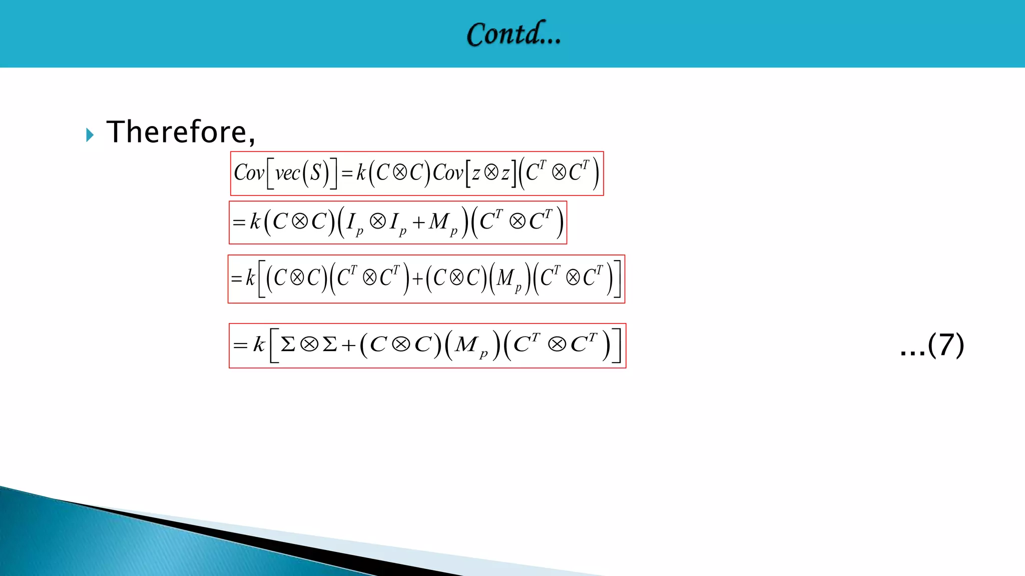
21.  Applying the vector(vec) operator to S, which forms a long vector
by stacking the columns of S, so that Cov[vec(s)] is a matrix rather
than an array, so we have
  k   T T Cov vec S   Cov vec Czz C   
    T  kCov  CC vec zz 
 
     T T k C C Cov vec zz  C C
  
 
     T T  k CC Cov zz C C
(by the vec to Kronecker property)
(by vec and Kronecker properties)
z

22.  To determine cov [vec(s)] (as a proxy for cov(s)), one would only
need to know
Covzz
(1) The variance of (where n is any element of z);
(2) The variance of Z Z (where no
are any two elements of z);
n o (3) The covariance between & ;
2
n Z 2
(4) The covariance between & and
o Z
(5) The covariance between and (where at most two of i, j, n, or
o are the same).
n o ZZ o n ZZ
n o Z Z
2
n Z

23. 1. is standard normally distributed, so follows a distribution
variance equal to 2(1) = 2. Therefore, = 2 for all k.
n Z
2. & are uncorrelated standard normal random variables, which
implies that they are also independent. Therefore,
due to independence
Here & both follow a distribution.
2 ) (1
              2 2 2 2 2 0 n o n o n o Var Z Z  E  Z Z   E Z E Z  E Z Z   E Z E Z
 
2 2 ( ) ( )( ) 1 1 1 n o n o Var Z Z  E Z Z   
2  (1)
n Z
2 ()n VZ

24. 3. & uncorrelated standard normal random variables,
         2 2   2  2 — — 1— 0 1 n o o n n o o n n o o n n o n o Cov Z Z Z Z  E Z Z Z Z E Z Z E Z Z  E Z Z E Z E Z  
so
4.       2 2 2 2 2 2 ( , ) — 1 1 0 n o n o n o Cov Z Z  E Z Z E Z E Z   
5.  ,  0 i j n o Cov Z Z Z Z 

25. Therefore, the [p(n-1)+ n,p(n -1)+n] elements of will all be 2
because Var  Z 2  
2 and the remaining diagonal elements of
k will all be 1 because Var  Z Z  
1 n o for all k = l. The off-diagonal elements
must be 0 except for those elements symbolizing the covariance
between ZZ and ZZ
j i , which will be 1.
i j Ultimately can be written as
i j Z Z j i Z Z
is a matrix of 1s and 0s.
I p I p Mp 
p M 2 2 p  p
2 2 p p  p M

26.  Therefore,
     Cov vec S   k CC Cov zz CT CT 
    T T
p p p  k CC I I M C C
       T T T T
p  k  CC C C  CC M C C 
 
     T T
  ...(7)
p  k   CC M C C 

27.  And we can check the derivation by simulating draws from a
Wishart distribution and comparing the simulated covariance with
the empirical covariance matrix calculated using equation (7).
 Analysis is done with the help of R console.

28.  Results shows that replications must be very large to be for the
empirical covariance matrix to be close to the theoretical covariance
matrix.

29. Some Theorems of Wishart Distribution

30. Some Theorems on Wishart Distribution

31.  Wishart distribution have great importance in the estimation of
covariance matrices in multivariate statistics.
 The Wishart distribution is frequently used as the prior on the
precision matrix parameter of a multivariate normal distribution.
 The Wishart distribution arises as models for random variation and
descriptions of uncertainty about variance and precision matrices. They
are of particular interest in sampling and inference on covariance and
association structure in multivariate normal models, and in ranges of
extensions in regression.

32.  The Inverse-Wishart distribution is the multivariate extension of the
Inverse-Gamma distribution.
 Even though the Wishart distribution generates sums of squares
matrices, one can think of the Inverse-Wishart distribution as
generating random covariance matrices.
 However, those covariance matrices would be inverses of the
covariance matrices generated underWishart distribution.

33.  Let T ~ InvWishp
Where denotes a positive definite scale matrix, m denotes the degrees of
freedom, and p indicates the dimensions of T (i.e. ).
Then T is positive definite with probability density function is given as
m
|Ψ| 2 1 = exp[- tr(ΨT-1)]
  ...(8)
m+p+1 mp 2
2 2 m | T | 2 Γp( )
f
2
T =
( , ) m 
Ψ
p×p TR

34.  The expected value of T is
...(9)
T
 ( )


m p
 
1
 In respect to the distribution, the only differences between the
2 Inverse-Wishart expectation and the inverse- χ
expectation are the
dimensionality of the data and a scale component.
 The Inverse-Wishart distribution has finite expectation only when m >
(p -1).

35.  The variance of the ijth element of T is
2
m p m p
( 1) ( 1)
       
ij ii jj
2
(T )
m p m p m p
( )( 1) ( 3)
ij
Var

    
ij ψ
Where is the element of the matrix
If p = 1, then only element of the variance/covariance matrix is given by
2
11 11   1
 The variance expression is given by
m m m
( )  1  (  2)  1  1 2( 
1) 2
  
2 2 2
Var X
( )
m m m m m m m m
(  1)(  2) (  4) (  1)(  2) (  4) (  2) ( 
4)
Inv-χ2(m)
Which is same as the variance of variable.

36.  The Wishart distribution is related to the normal distribution, Chi-square
distribution and Gamma distribution . The Inverse-Wishart distribution
is related to the those distributions in a similar way.
let
~ (k, ) p S W 
1 1 ~ ( , ) p S InvWish m   
then
Where m=k is the degrees of freedom

39.  The Inverse-Wishart distribution is frequently used as the prior on
the variance/covariance matrix parameter (S) of a multivariate
normal distribution. Note that the Inverse-Gamma distribution is the
conjugate prior for the variance parameter of a univariate normal
distribution, and the Inverse-Wishart distribution (as its multivariate
generalization) extends conjugacy to the multivariate normal
distribution.

40.  The Wishart and Inverse-Wishart distribution is an important
distribution having a certain good and useful statistical properties.
These distributions have important role in estimating parameter in
multivariate studies.
 Wishart distribution help to develop a framework for bayesian
inference for Gaussian covariance graph models.
 Hence this work completes the powerful theory that has been developed
in the mathematical statistics literature for decomposable models. This
models help to draw a valid inference.

41. Conclusion:
 The generalized Wishart process (GWP) – which we used to model
time-varying covariance matrices σ(t). In the future, the GWP could be
applied to study how Σ depends on covariates like interest rates.

42. Anderson, T. W.(2003). An Introduction to Multivariate Statistical
Analysis. Wiley India (P) Ltd., New Delhi.
Chatfield, C. and Collins, A. J.(1980). Introduction to Multivariate
Analysis. Chapman and Hall-CRC, London.
Chib, S. and Greenberg, E.(1998). Bayesian analysis of multivariate
probit models. Biometrika , 85, 347-361.
Cook, R. D.(2011). On the mean and variance of the generalized
inverse of a singular Wishart matrix . Electronic Journal of Statistics
, 5, 146-158.

43. Eaton, M. L.(2007). Multivariate statistics: A vector space approach , .
Wiley India (P) Ltd., New Delhi.
Nydick, S. W.(2012). The Wishart and inverse Wishart distributions.
International Journal of Electronics and Communication,
22, 119-139.
Pourahmadi, M., Daniels, M. J. and Park, T.(2006). Simultaneously
modelling of the cholesky decomposition of several covariance
matrices. Journal of Multivariate Analysis, 97, 125-135.

44. Rao, C. R.(1965). Linear statistical inference and its applications,
Wiley India (P) Ltd., New Delhi.

46. Cholesky decomposition
It is a decomposition of hermitian positive definite
matrix into the product of lower triangular matrix
and it conjugate transpose.
The cholesky decomposition of a hermitian positive-definite
matrix a is a decomposition of the form.
A LL 
Where L is a lower triangular matrix with real and
positive diagonal entries, and L* denotes the
conjugate transpose of L

47. R CODE

48. M

49. Any
Question
s ????