Download as PDF, PPTX


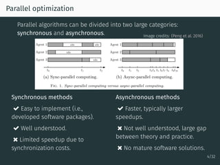

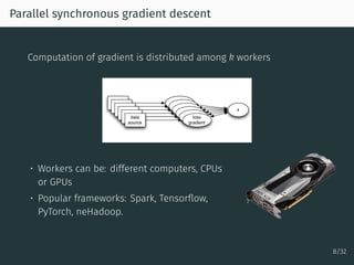

![Unbiased gradient estimate
SGD-like algorithms crucially rely on the unbiased property
Ei[∇fi(x)] = ∇f(x).
For synchronous algorithms, follows from the uniform sampling of i
Ei[∇fi(x)] =
n∑
i=1
Proba(selecting i)∇fi(x)
uniform sampling
=
n∑
i=1
1
n
∇fi(x) = ∇f(x)
16/32](https://image.slidesharecdn.com/mc10-pedregosa-171220193838/85/Parallel-Optimization-in-Machine-Learning-28-320.jpg)
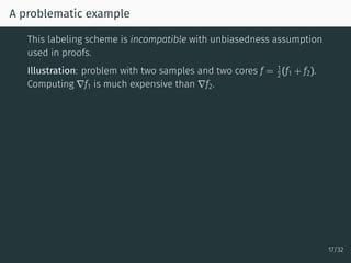
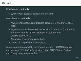
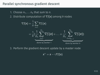
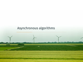
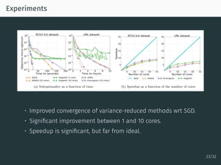
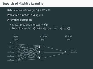
![A problematic example
This labeling scheme is incompatible with unbiasedness assumption
used in proofs.
Illustration: problem with two samples and two cores f = 1
2 (f1 + f2).
Computing ∇f1 is much expensive than ∇f2.
Start at x0. Because of the random sampling there are 4 possible
scenarios:
1. Core 1 selects f1, Core 2 selects f1 =⇒ x1 = x0 − γ∇f1(x)
2. Core 1 selects f1, Core 2 selects f2 =⇒ x1 = x0 − γ∇f2(x)
3. Core 1 selects f2, Core 2 selects f1 =⇒ x1 = x0 − γ∇f2(x)
4. Core 1 selects f2, Core 2 selects f2 =⇒ x1 = x0 − γ∇f2(x)
So we have
Ei [∇fi] =
1
4
f1 +
3
4
f2
̸=
1
2
f1 +
1
2
f2 !!
17/32](https://image.slidesharecdn.com/mc10-pedregosa-171220193838/85/Parallel-Optimization-in-Machine-Learning-31-320.jpg)


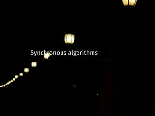
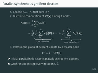
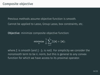
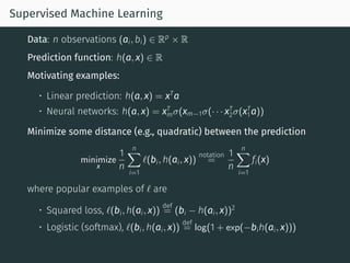
![The SAGA algorithm
Setting:
minimize
x
1
n
n∑
i=1
fi(x)
The SAGA algorithm (Defazio, Bach, and Lacoste-Julien 2014).
Select i ∈ {1, . . . , n} and compute (x+
, α+
) as
x+
= x − γ(∇fi(x) − αi + α) ; α+
i = ∇fi(x)
• Like SGD, update is unbiased, i.e., Ei[∇fi(x) − αi + α)] = ∇f(x).
• Unlike SGD, because of memory terms α, variance → 0.
• Unlike SGD, converges with fixed step size (1/3L)
19/32](https://image.slidesharecdn.com/mc10-pedregosa-171220193838/85/Parallel-Optimization-in-Machine-Learning-36-320.jpg)
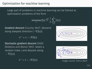
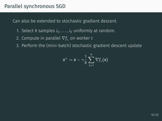
![The SAGA algorithm
Setting:
minimize
x
1
n
n∑
i=1
fi(x)
The SAGA algorithm (Defazio, Bach, and Lacoste-Julien 2014).
Select i ∈ {1, . . . , n} and compute (x+
, α+
) as
x+
= x − γ(∇fi(x) − αi + α) ; α+
i = ∇fi(x)
• Like SGD, update is unbiased, i.e., Ei[∇fi(x) − αi + α)] = ∇f(x).
• Unlike SGD, because of memory terms α, variance → 0.
• Unlike SGD, converges with fixed step size (1/3L)
Super easy to use in scikit-learn
19/32](https://image.slidesharecdn.com/mc10-pedregosa-171220193838/85/Parallel-Optimization-in-Machine-Learning-37-320.jpg)
![Sparse SAGA
Need for a sparse variant of SAGA
• A large part of large scale datasets are sparse.
• For sparse datasets and generalized linear models (e.g., least
squares, logistic regression, etc.), partial gradients ∇fi are sparse
too.
• Asynchronous algorithms work best when updates are sparse.
SAGA update is inefficient for sparse data
x+
= x − γ(∇fi(x)
sparse
− αi
sparse
+ α
dense!
) ; α+
i = ∇fi(x)
[scikit-learn uses many tricks to make it efficient that we cannot use
in asynchronous version]
20/32](https://image.slidesharecdn.com/mc10-pedregosa-171220193838/85/Parallel-Optimization-in-Machine-Learning-38-320.jpg)
![Sparse SAGA
Sparse variant of SAGA. Relies on
• Diagonal matrix Pi = projection onto the support of ∇fi
• Diagonal matrix D defined as
Dj,j = n/number of times ∇jfi is nonzero.
Sparse SAGA algorithm (Leblond, P., and Lacoste-Julien 2017)
x+
= x − γ(∇fi(x) − αi + PiDα) ; α+
i = ∇fi(x)
• All operations are sparse, cost per iteration is
O(nonzeros in ∇fi).
• Same convergence properties than SAGA, but with cheaper
iterations in presence of sparsity.
• Crucial property: Ei[PiD] = I.
21/32](https://image.slidesharecdn.com/mc10-pedregosa-171220193838/85/Parallel-Optimization-in-Machine-Learning-39-320.jpg)

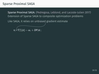
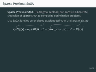
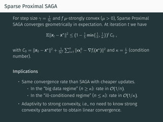
![Sparse Proximal SAGA
Sparse Proximal SAGA. (Pedregosa, Leblond, and Lacoste-Julien 2017)
Extension of Sparse SAGA to composite optimization problems
Like SAGA, it relies on unbiased gradient estimate and proximal step
vi=∇fi(x) − αi + DPiα ; x+
= proxγφi
(x − γvi) ; α+
i = ∇fi(x)
Where Pi, D are as in Sparse SAGA and φi
def
=
∑d
j (PiD)i,i|xj|.
φi has two key properties: i) support of φi = support of ∇fi (sparse
updates) and ii) Ei[φi] = ∥x∥1 (unbiasedness)
26/32](https://image.slidesharecdn.com/mc10-pedregosa-171220193838/85/Parallel-Optimization-in-Machine-Learning-48-320.jpg)
![Sparse Proximal SAGA
Sparse Proximal SAGA. (Pedregosa, Leblond, and Lacoste-Julien 2017)
Extension of Sparse SAGA to composite optimization problems
Like SAGA, it relies on unbiased gradient estimate and proximal step
vi=∇fi(x) − αi + DPiα ; x+
= proxγφi
(x − γvi) ; α+
i = ∇fi(x)
Where Pi, D are as in Sparse SAGA and φi
def
=
∑d
j (PiD)i,i|xj|.
φi has two key properties: i) support of φi = support of ∇fi (sparse
updates) and ii) Ei[φi] = ∥x∥1 (unbiasedness)
Convergence: same linear convergence rate as SAGA, with cheaper
updates in presence of sparsity.
26/32](https://image.slidesharecdn.com/mc10-pedregosa-171220193838/85/Parallel-Optimization-in-Machine-Learning-49-320.jpg)
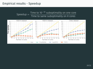
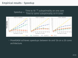
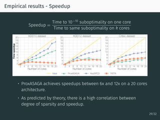


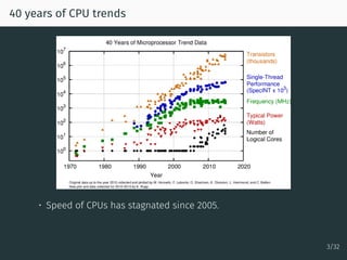
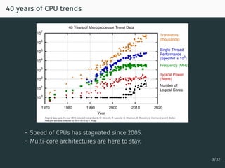
The document discusses parallel optimization in machine learning, focusing on the challenges and methodologies related to synchronous and asynchronous algorithms. It highlights the stagnation of CPU speed since 2005 and presents various optimization approaches, such as stochastic gradient descent and its asynchronous variants, including 'Hogwild' and 'SAGA'. Additionally, it introduces the 'sparse proximal SAGA' method for handling sparse datasets and composite optimization problems efficiently.


![Differential privacy without sensitivity [NIPS2016読み会資料]](https://cdn.slidesharecdn.com/ss_thumbnails/nipsyomi2016slideshare-170122091905-thumbnail.jpg?width=640&height=640&fit=bounds)