Download as PDF, PPTX

![R packages Potts model Bayesian computation Conclusion
Annotations
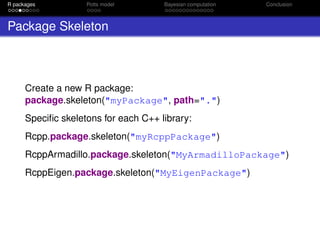
Rcpp wrappers generated automatically:
compileAttributes("myRcppPackage")
R package documentation generated automatically:
roxygenize("myRcppPackage")
§
/ / ’ Compute the effective sample size (ESS) of the particles.
/ / ’
/ / ’ The ESS is a ‘‘rule of thumb’’ for assessing the degeneracy of
/ / ’’ the importance distribution:
/ / ’ deqn {ESS = frac { ( sum_ { q=1}^Q w_q ) ^ 2 } { sum_ { q=1}^Q w_q ^2}}
/ / ’
/ / ’’ @param log_weights logarithms of the importance weights of each particle.
/ / ’’ @return the effective sample size, a scalar between 0 and Q
/ / ’’ @references
/ / ’’ Liu, JS (2001) "Monte Carlo Strategies in Scientific Computing." Springer’
/ / [ [ Rcpp : : export ] ]
double effectiveSampleSize ( NumericVector log_weights )
{
double sum_wt = sum_logs ( log_weights ) ;
double sum_sq = sum_logs ( log_weights + log_weights ) ;
double res = exp (sum_wt + sum_wt − sum_sq ) ;
i f ( std : : i s f i n i t e ( res ) ) return res ;
else return 0;
}](https://image.slidesharecdn.com/mtm20161202oxwasp-161202191907/85/R-package-bayesImageS-a-case-study-in-Bayesian-computation-using-Rcpp-and-OpenMP-7-320.jpg)

![R packages Potts model Bayesian computation Conclusion
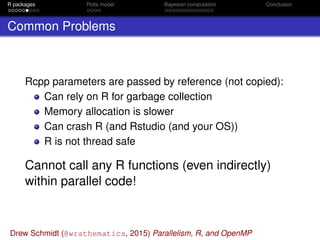
Gibbs sampler in C++
§
void gibbsLabels ( const arma : : umat & neigh , const std : : vector <arma : : uvec> & blocks ,
arma : : umat & z , arma : : umat & alloc , const double beta ,
const arma : : mat & log_ x f i e l d )
{
const Rcpp : : NumericVector randU = Rcpp : : r u n i f ( neigh . n_rows ) ;
for ( unsigned b=0; b < blocks . size ( ) ; b++)
{
const arma : : uvec block = blocks [ b ] ;
arma : : vec log_prob ( z . n_cols ) ;
#pragma omp p a r a l l e l for private ( log_prob )
for ( unsigned i =0; i < block . size ( ) ; i ++)
{
for ( unsigned j =0; j < z . n_cols ; j ++)
{
unsigned sum_neigh = 0;
for ( unsigned k=0; k < neigh . n_cols ; k++)
{
sum_neigh += z ( neigh ( block [ i ] , k ) , j ) ;
}
log_prob [ j ] = log_ x f i e l d ( block [ i ] , j ) + beta∗sum_neigh ;
}
double t o t a l _ l l i k e = sum_logs ( log_prob ) ;
double cumProb = 0.0;
z . row ( block [ i ] ) . zeros ( ) ;
for ( unsigned j =0; j < log_prob . n_elem ; j ++)
{
cumProb += exp ( log_prob [ j ] − t o t a l _ l l i k e ) ;
i f ( randU [ block [ i ] ] < cumProb )
{
z ( block [ i ] , j ) = 1;
a l l o c ( block [ i ] , j ) += 1;
break ;](https://image.slidesharecdn.com/mtm20161202oxwasp-161202191907/85/R-package-bayesImageS-a-case-study-in-Bayesian-computation-using-Rcpp-and-OpenMP-18-320.jpg)
![R packages Potts model Bayesian computation Conclusion
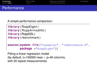
Pseudolikelihood (PL)
Algorithm 2 Metropolis-Hastings with PL
1: Draw proposal β ∼ q(β |β◦)
2: Approximate p(β |z) and p(β◦|z) using equation (7):
ˆpPL(β|z) ≈
n
i=1
exp{β i∼ δ(zi, z )}
k
j=1 exp{β i∼ δ(j, z )}
(7)
3: Calculate the M-H ratio ρ = ˆpPL(β |z)π(β )q(β◦|β )
ˆpPL(β◦|z)π(β◦)q(β |β◦)
4: Draw u ∼ Uniform[0, 1]
5: if u < min(1, ρ) then
6: β ← β
7: else
8: β ← β◦
9: end if
Rydén & Titterington (1998) JCGS 7(2): 194–211](https://image.slidesharecdn.com/mtm20161202oxwasp-161202191907/85/R-package-bayesImageS-a-case-study-in-Bayesian-computation-using-Rcpp-and-OpenMP-19-320.jpg)
![R packages Potts model Bayesian computation Conclusion
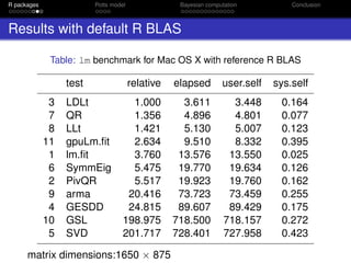
Pseudolikelihood in C++
§
double pseudolike ( const arma : : mat & ne , const arma : : uvec & e , const double b ,
const unsigned n , const unsigned k )
{
double num = 0.0;
double denom = 0.0;
#pragma omp p a r a l l e l for reduction ( + :num, denom)
for ( unsigned i =0; i < n ; i ++)
{
num=num+ne ( e [ i ] , i ) ;
double tdenom =0.0;
for ( unsigned j =0; j < k ; j ++)
{
tdenom=tdenom+exp ( b∗ne ( j , i ) ) ;
}
denom=denom+log ( tdenom ) ;
}
return b∗num−denom ;
}](https://image.slidesharecdn.com/mtm20161202oxwasp-161202191907/85/R-package-bayesImageS-a-case-study-in-Bayesian-computation-using-Rcpp-and-OpenMP-20-320.jpg)
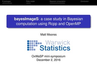
![R packages Potts model Bayesian computation Conclusion
Thermodynamic Integration (TI)
Path sampling identity:
log
C(β◦)
C(β )
=
β◦
β
E z|β [S(z)] dβ (8)
0.0 0.5 1.0 1.5 2.0
500000100000015000002000000
ϕ
S(x)
Gelman & Meng (1998) Stat. Sci. 13(2): 163–185.](https://image.slidesharecdn.com/mtm20161202oxwasp-161202191907/85/R-package-bayesImageS-a-case-study-in-Bayesian-computation-using-Rcpp-and-OpenMP-22-320.jpg)
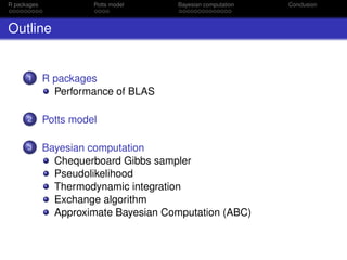
![R packages Potts model Bayesian computation Conclusion
TI algorithm
Algorithm 3 Random walk Metropolis with TI
1: Draw random walk proposal β ∼ q(β |β◦)
2: Estimate S(z|β◦) and S(z|β ) by interpolation
3: Evaluate the definite integral in equation (8)
4: Calculate the log M-H acceptance ratio:
log{ρ} = log
C(β◦)
C(β )
+ (β − β◦
)S(z) (9)
5: Draw u ∼ Uniform[0, 1]
6: if u < min(1, ρ) then
7: β ← β
8: else
9: β ← β◦
10: end if](https://image.slidesharecdn.com/mtm20161202oxwasp-161202191907/85/R-package-bayesImageS-a-case-study-in-Bayesian-computation-using-Rcpp-and-OpenMP-23-320.jpg)
![R packages Potts model Bayesian computation Conclusion
TI in C++
§
unsigned pathBeta ( const arma : : umat & neigh , const std : : vector <arma : : uvec> & blocks ,
const arma : : mat & path , const arma : : umat & z , double & beta ,
const double p r i o r _beta [ 2 ] , const double bw)
{
double bprime = rwmh( beta , bw, p r i o r _beta ) ; / / truncated Gaussian
/ / approximate log (Z( bprime ) / Z( beta ) )
double log_ r a t i o = quadrature ( bprime , beta , path )
+ ( bprime−beta ) ∗ sum_ ident ( z , neigh , blocks ) ;
/ / accept / r e j e c t
i f ( u n i f _rand ( ) < exp ( log_ r a t i o ) )
{
beta = bprime ;
return 1;
}
return 0;
}](https://image.slidesharecdn.com/mtm20161202oxwasp-161202191907/85/R-package-bayesImageS-a-case-study-in-Bayesian-computation-using-Rcpp-and-OpenMP-24-320.jpg)
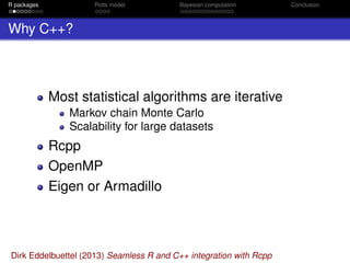
![R packages Potts model Bayesian computation Conclusion
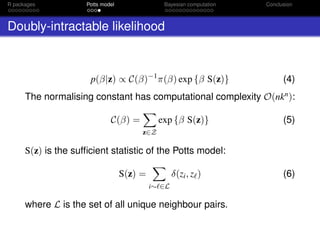
Approximate Exchange Algorithm (AEA)
Algorithm 4 AEA
1: Draw random walk proposal β ∼ q(β |β◦)
2: Generate w|β by sampling from eq. (3)
3: Calculate the M-H acceptance ratio according to eq. (4):
ρ =
π(β ) exp {β S(z)} C(β◦)
π(β◦) exp {β◦S(z)} C(β )
exp {β◦S(w)} C(β )
exp {β S(w)} C(β◦)
(10)
4: Draw u ∼ Uniform[0, 1]
5: if u < min(1, ρ) then
6: β ← β
7: else
8: β ← β◦
9: end if
Murray, Ghahramani & MacKay (2006) Proc. 22nd
Conf. UAI, 359–366](https://image.slidesharecdn.com/mtm20161202oxwasp-161202191907/85/R-package-bayesImageS-a-case-study-in-Bayesian-computation-using-Rcpp-and-OpenMP-25-320.jpg)
![R packages Potts model Bayesian computation Conclusion
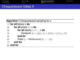
AEA in C++
§
unsigned exchangeBeta ( const arma : : umat & neigh , const std : : vector <arma : : uvec> & blocks ,
const arma : : uvec & slice , const arma : : umat & z , double & beta ,
const double p r i o r _beta [ 2 ] , const unsigned aux , const bool useSW,
const bool swapAux , const double bw)
{
double bprime = rwmh( beta , bw, p r i o r _beta ) ;
arma : : umat a l l o c = arma : : zeros <arma : : umat >(z . n_rows−1, z . n_cols ) ;
arma : : umat w;
i f ( swapAux ) w = z ;
else w = randomIndices ( z . n_rows−1, z . n_cols ) ;
for ( unsigned i =0; i <aux ; i ++)
{
i f (useSW)
{
swLabelsNoData ( neigh , blocks , bprime , w. n_cols , w, a l l o c ) ;
}
else
{
gibbsLabelsNoData ( neigh , blocks , w, alloc , bprime ) ;
}
}
double sum_z = sum_ ident ( z , neigh , blocks ) ;
double sum_w = sum_ ident (w, neigh , blocks ) ;
double log_ r a t i o = ( bprime−beta )∗sum_z + ( beta−bprime )∗sum_w;
/ / accept / r e j e c t
i f ( u n i f _rand ( ) < exp ( log_ r a t i o ) )
{
beta = bprime ;
return 1;
}
return 0;
}](https://image.slidesharecdn.com/mtm20161202oxwasp-161202191907/85/R-package-bayesImageS-a-case-study-in-Bayesian-computation-using-Rcpp-and-OpenMP-26-320.jpg)
![R packages Potts model Bayesian computation Conclusion
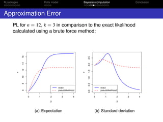
ABC with Metropolis-Hastings
Algorithm 6 ABC-MCMC
1: Draw proposal β ∼ q(β |β◦)
2: Generate w|β by sampling from eq. (3)
3: Draw u ∼ Uniform[0, 1]
4: if u < π(β )q(β◦|β )
π(β◦)q(β |β◦) and S(w) − S(z) < then
5: β ← β
6: else
7: β ← β◦
8: end if
Marjoram, Molitor, Plagnol & Tavaré (2003) PNAS 100(26): 15324–28](https://image.slidesharecdn.com/mtm20161202oxwasp-161202191907/85/R-package-bayesImageS-a-case-study-in-Bayesian-computation-using-Rcpp-and-OpenMP-28-320.jpg)
![R packages Potts model Bayesian computation Conclusion
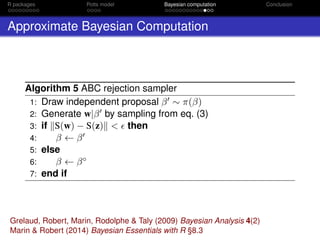
ABC-MCMC in C++
§
unsigned abcBeta ( const arma : : umat & neigh , const std : : vector <arma : : uvec> & blocks ,
const arma : : umat & z , double & beta , const double p r i o r _beta [ 2 ] ,
const unsigned aux , const bool useSW, const bool swapAux ,
const double bw, const double epsilon )
{
double bprime = rwmh( beta , bw, p r i o r _beta ) ;
arma : : umat a l l o c = arma : : zeros <arma : : umat >(z . n_rows−1, z . n_cols ) ;
arma : : umat w;
i f ( swapAux ) w = z ;
else w = randomIndices ( z . n_rows−1, z . n_cols ) ;
for ( unsigned i =0; i <aux ; i ++)
{
i f (useSW)
{
swLabelsNoData ( neigh , blocks , bprime , w. n_cols , w, a l l o c ) ;
}
else
{
gibbsLabelsNoData ( neigh , blocks , w, alloc , bprime ) ;
}
}
double sum_z = sum_ ident ( z , neigh , blocks ) ;
double sum_w = sum_ ident (w, neigh , blocks ) ;
double delta = fabs (sum_w − sum_z ) ;
i f ( delta < epsilon )
{
beta = bprime ;
return 1;
}
return 0;
}](https://image.slidesharecdn.com/mtm20161202oxwasp-161202191907/85/R-package-bayesImageS-a-case-study-in-Bayesian-computation-using-Rcpp-and-OpenMP-29-320.jpg)
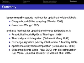

![Appendix
For Further Reading II
M. Moores & K. Mengersen
bayesImageS: Bayesian methods for image segmentation using a
hidden Potts model.
R package version 0.3-3
https://CRAN.R-project.org/package=bayesImageS
M. Moores, A. N. Pettitt & K. Mengersen
Scalable Bayesian inference for the inverse temperature of a hidden
Potts model.
arXiv:1503.08066 [stat.CO], 2015.
M. Moores, C. C. Drovandi, K. Mengersen & C. P. Robert
Pre-processing for approximate Bayesian computation in image
analysis.
Statistics & Computing 25(1): 23–33, 2015.
M. Moores & K. Mengersen
Bayesian approaches to spatial inference: modelling and computational
challenges and solutions.
In Proc. 33rd Int. Wkshp MaxEnt, AIP Conf. Proc. 1636: 112–117, 2014.](https://image.slidesharecdn.com/mtm20161202oxwasp-161202191907/85/R-package-bayesImageS-a-case-study-in-Bayesian-computation-using-Rcpp-and-OpenMP-33-320.jpg)

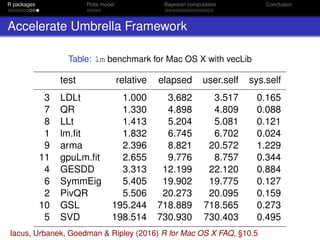
This document discusses the use of R packages for Bayesian computation, particularly in the context of the Potts model and associated computational methods such as Gibbs sampling and Monte Carlo techniques. It emphasizes the integration of C++ with R for enhanced performance, outlines package creation and documentation, and provides insight into various algorithms used in Bayesian analysis. The document includes benchmarks and comparisons of different statistical algorithms utilizing R and C++.


![谷歌留痕技术 [ 𝙩𝙤𝙥 𝟮𝟯𝟯. 𝙘 𝙤𝙢 ]](https://cdn.slidesharecdn.com/ss_thumbnails/top233-260130174328-3833018c-thumbnail.jpg?width=640&height=640&fit=bounds)


