Download as PDF, PPTX
![GRADIENT-BASED HYPERPARAMETER OPTIMIZATION
Compute gradients with respect to hyperparameters
[Larsen 1996, 1998, Bengio 2000].
Hyperparameter optimization as nested or bi-level
optimization:
arg min
λ∈
s.t. X(λ)
⏟model parameters
f (λ) ≜ g(X(λ), λ)
loss on test set
∈ arg min
x∈ℝp
h(x, λ)
⏟loss on train set](https://image.slidesharecdn.com/icmltalk-160620125922/85/Hyperparameter-optimization-with-approximate-gradient-4-320.jpg)
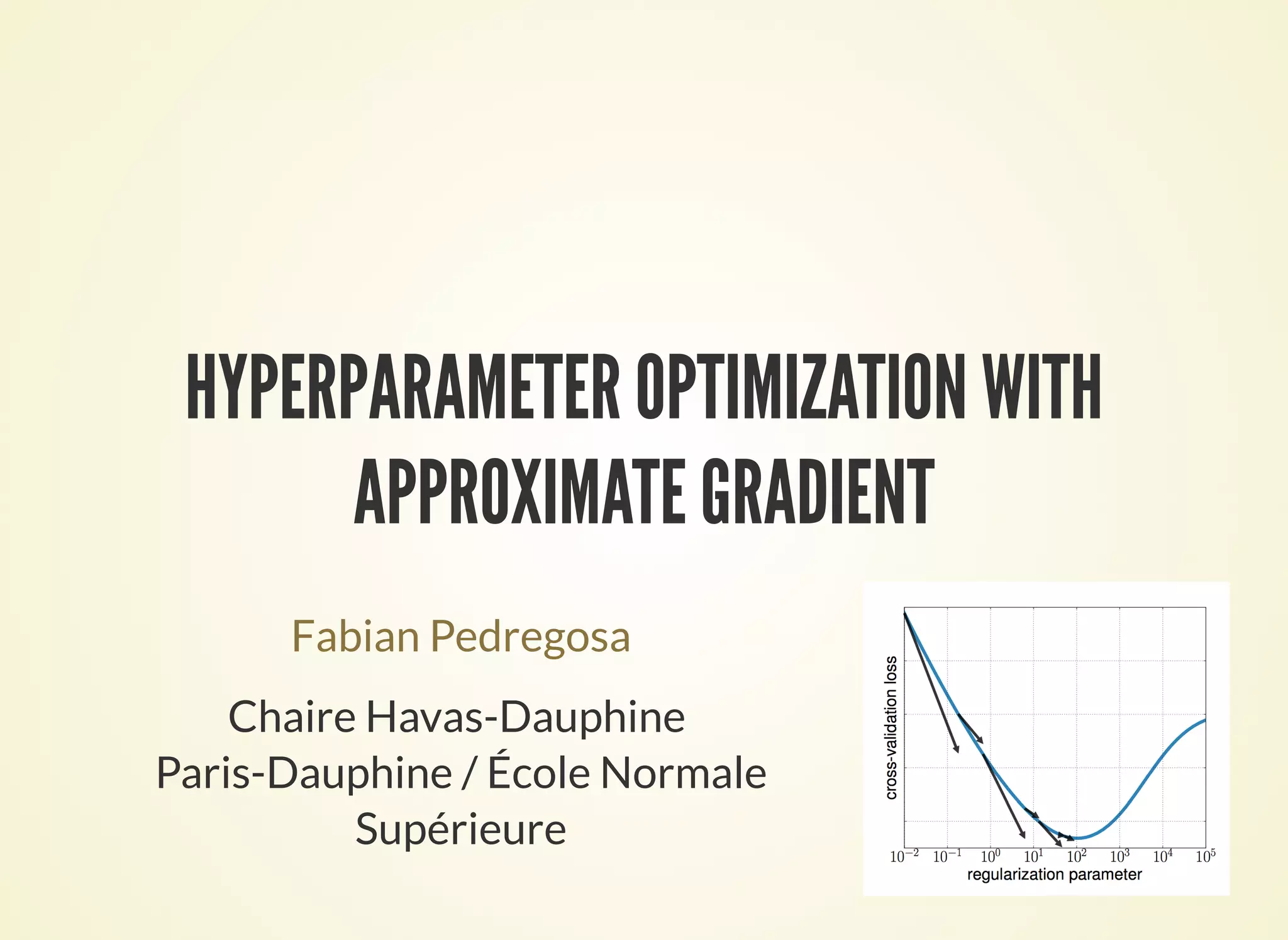
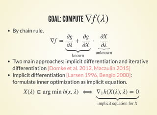
![GOAL: COMPUTE ∇f (λ)
By chain rule,
Two main approaches: implicit differentiation and iterative
differentiation [Domke et al. 2012, Macaulin 2015]
Implicit differentiation [Larsen 1996, Bengio 2000]:
formulate inner optimization as implicit equation.
∇f = ⋅+
∂g
∂λ
∂g
∂X
known
∂X
∂λ
⏟unknown
X(λ) ∈ arg min h(x, λ) ⟺ h(X(λ), λ) = 0∇1
implicit equation for X](https://image.slidesharecdn.com/icmltalk-160620125922/85/Hyperparameter-optimization-with-approximate-gradient-5-320.jpg)
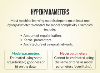
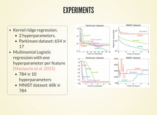
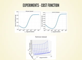
![EXPERIMENTS II
Kernel ridge regression.
2 hyperparameters.
Parkinson dataset: 654
17
Multinomial Logistic
regression with one
hyperparameter per feature
[Maclaurin et al. 2015]
784 10
hyperparameters
MNIST dataset: 60k
784
×
×
×](https://image.slidesharecdn.com/icmltalk-160620125922/85/Hyperparameter-optimization-with-approximate-gradient-12-320.jpg)
![REFERENCES
[Y. Bengio, 2000] Bengio, Yoshua. "Gradient-based optimization of
hyperparameters." Neural computation 12.8 (2000): 1889-1900.
[J. Bergstra, Y. Bengio 2012] Bergstra, James, and Yoshua Bengio. "Random
search for hyper-parameter optimization." The Journal of Machine
Learning Research 13.1 (2012): 281-305.
[J. Snoek et al., 2015] Snoek, J. et al. Scalable Bayesian Optimization Using
Deep Neural Networks. (2015). at
[K. Swersky et al., 2014] Swersky, K., Snoek, J. & Adams, R. Freeze-Thaw
Bayesian Optimization. arXiv Prepr. arXiv1406.3896 1–12 (2014). at
[F. Hutter et al., 2013] Hutter, F., Hoos, H. & Leyton-Brown, K. An
evaluation of sequential model-based optimization for expensive blackbox
functions.
http://arxiv.org/abs/1502.05700a
http://arxiv.org/abs/1406.3896](https://image.slidesharecdn.com/icmltalk-160620125922/85/Hyperparameter-optimization-with-approximate-gradient-14-320.jpg)
![REFERENCES 2
[M. Schmidt et al., 2013] Schmidt, M., Roux, N. & Bach, F. Minimizing nite
sums with the stochastic average gradient. arXiv Prepr. arXiv1309.2388
1–45 (2013). at
[J. Domke et al., 2012] Domke, J. Generic Methods for Optimization-Based
Modeling. Proc. Fifteenth Int. Conf. Artif. Intell. Stat. XX, 318–326 (2012).
[M. P. Friedlander et al., 2012] Friedlander, M. P. & Schmidt, M. Hybrid
Deterministic-Stochastic Methods for Data Fitting. SIAM J. Sci. Comput.
34, A1380–A1405 (2012).
http://arxiv.org/abs/1309.2388](https://image.slidesharecdn.com/icmltalk-160620125922/85/Hyperparameter-optimization-with-approximate-gradient-15-320.jpg)

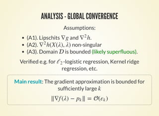
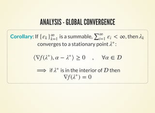
This document discusses hyperparameter optimization using approximate gradients. It introduces the problem of optimizing hyperparameters along with model parameters. While model parameters can be estimated from data, hyperparameters require methods like cross-validation. The document proposes using approximate gradients to optimize hyperparameters more efficiently than costly methods like grid search. It derives the gradient of the objective with respect to hyperparameters and presents an algorithm called HOAG that approximates this gradient using inexact solutions. The document analyzes HOAG's convergence and provides experimental results comparing it to other hyperparameter optimization methods.


![谷歌留痕技术 [ 𝙩𝙤𝙥 𝟮𝟯𝟯. 𝙘 𝙤𝙢 ]](https://cdn.slidesharecdn.com/ss_thumbnails/top233-260130174328-3833018c-thumbnail.jpg?width=640&height=640&fit=bounds)


