Download as PDF, PPTX


![Introduction Scalable Computation Informative Priors Conclusion
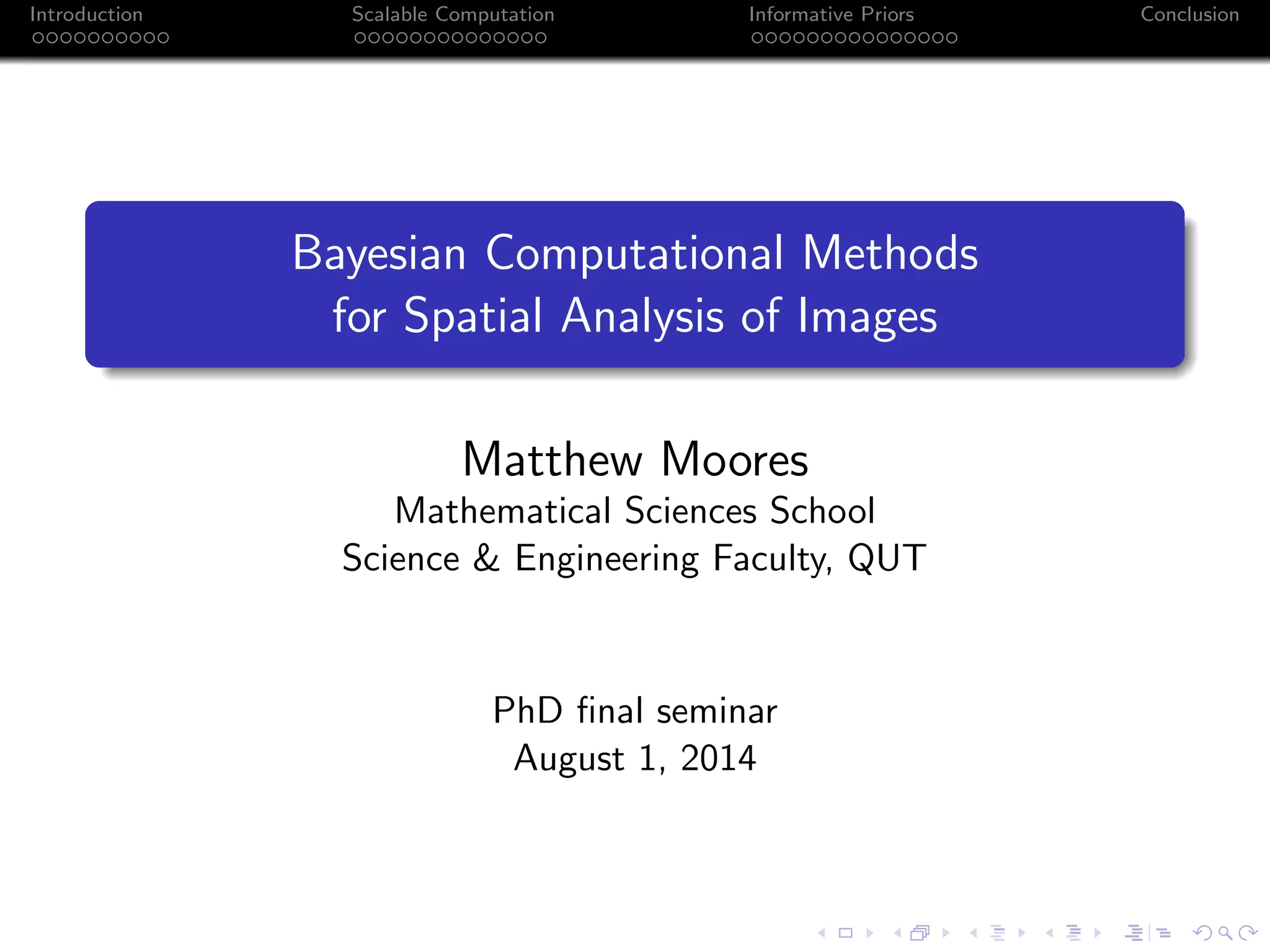
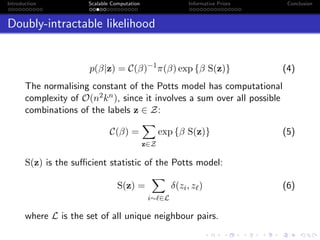
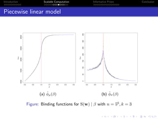
Expectation of S(z)
exact expectation of S(z) for n=12 and k=
β
E(S(z))
5
10
15
1 2 3 4
2
3
4
(a) n = 12 & k ∈ 2, 3, 4
exact expectation of S(z) for k=3 and n=
β
E(S(z))
5
10
15
1 2 3 4
4
6
9
12
(b) k = 3 & n ∈ 4, 6, 9, 12
Figure: Distribution of Ez|β[S(z)]](https://image.slidesharecdn.com/mooresphd-150603175634-lva1-app6892/85/Final-PhD-Seminar-18-320.jpg)
![Introduction Scalable Computation Informative Priors Conclusion
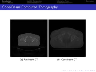
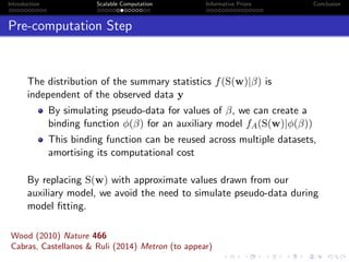
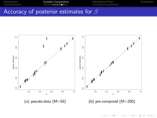
Standard deviation of S(z)
exact standard deviation of S(z) for n=12 and k=
β
σ(S(z))
0.0
0.5
1.0
1.5
2.0
2.5
3.0
1 2 3 4
2
3
4
(a) n = 12 & k ∈ 2, 3, 4
exact standard deviation of S(z) for k=3 and n=
β
σ(S(z))
0.0
0.5
1.0
1.5
2.0
2.5
1 2 3 4
4
6
9
12
(b) k = 3 & n ∈ 4, 6, 9, 12
Figure: Distribution of σz|β[S(z)]](https://image.slidesharecdn.com/mooresphd-150603175634-lva1-app6892/85/Final-PhD-Seminar-19-320.jpg)


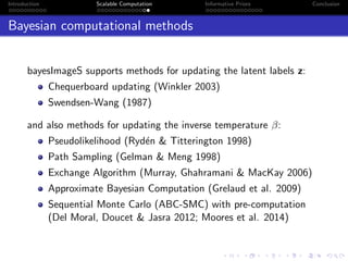


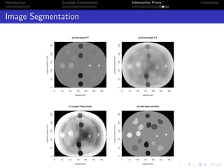

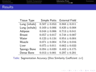
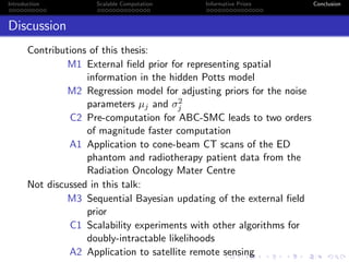

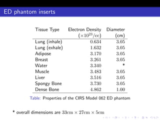


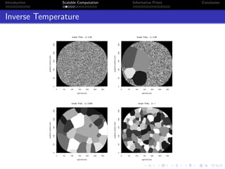
- The document summarizes Matthew Moores' PhD research on developing Bayesian computational methods for spatial analysis of medical and satellite images. - The objectives are to develop a generative image model incorporating prior information, implement it computationally efficiently, and apply it to radiotherapy and remote sensing data. - Challenges include intractable likelihoods, which are addressed through approximate Bayesian computation and sequential Monte Carlo with pre-computation. - The research aims to classify pixels in medical and satellite images according to tissue type or land use by incorporating informative priors.


![Inference in generative models using the Wasserstein distance [[INI]](https://cdn.slidesharecdn.com/ss_thumbnails/inewton-170706120746-thumbnail.jpg?width=640&height=640&fit=bounds)