update equations derivation for Poisson factorization in topic modeling

1. Topic modeling with Poisson factorization
Tomonari Masada @ Nagasaki University
February 3, 2017
1 ELBO
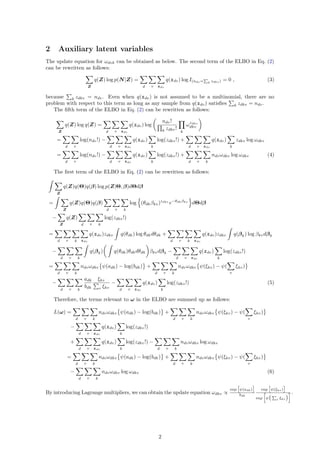
To obtain update equations, we introduce auxiliary latent variables Z [1, 2, 3, 4]. zdkv is the
number of the tokens of the vth word in the dth document assigned to the kth topic. zdkv is
sampled from the Poisson distribution Poisson(θdkβkv).
The constraint k zdkv = ndv can be expressed with the probability mass function I(ndv= k zdkv).
The full joint distribution is given as below.
p(N, Z, Θ, β; α, s, r) = p(β; α)p(Θ; s, r)p(N|Z)p(Z|Θ, β)
=
k
p(βk; α) ×
k
p(θk; sk, rk) ×
d
p(nd|zd)p(zd|θd, β)
=
k
Γ(V α)
Γ(α)V
v
βα−1
kv ×
k d
rsk
k
Γ(sk)
θsk−1
dk e−rkθdk
×
d v
I(ndv= k zdkv)
k
(θdkβkv)zdkv
e−θdkβkv
zdkv!
(1)
The generative model is fully described in Eq. (1).
We adopt the variational Bayesian inference for the posterior inference. The evidence lower
bound (ELBO) for the model is obtained as below.
log p(N) = log
Z
p(N, Z, Θ, β)dΘdβ
≥
Z
q(Z)q(Θ)q(β) log p(N, Z, Θ, β)dΘdβ −
Z
q(Z)q(Θ)q(β) log q(Z)q(Θ)q(β)dΘdβ
=
Z
q(Z)q(Θ)q(β) log p(Z|Θ, β)dΘdβ
+
Z
q(Z) log p(N|Z) + q(Θ) log p(Θ)dΘ + q(β) log p(β)dβ
−
z
q(Z) log q(Z) − q(Θ) log q(Θ)dΘ − q(β) log q(β)dβ , (2)
where the approximate posterior q(Z, Θ, β) is factorized.
We assume the followings for the factorized approximate posterior.
• q(zdv) is the multinomial distribution Mult(ndv, ωdv). ωdvk is the probability that a token
of the vth word in the dth document is assigned to the kth topic among the K topics. Note
that k zdkv = ndv holds.
• q(θdk) is the gamma distribution Gamma(adk, bdk).
• q(βk) is the asymmetric Dirichlet distribution Dirichlet(ξk).
1

2. 2 Auxiliary latent variables
The update equation for ωdvk can be obtained as below. The second term of the ELBO in Eq. (2)
can be rewritten as follows:
Z
q(Z) log p(N|Z) =
d v zdv
q(zdv) log I(ndv= k zdkv) = 0 , (3)
because k zdkv = ndv. Even when q(zdv) is not assumed to be a multinomial, there are no
problem with respect to this term as long as any sample from q(zdv) satisfies k zdkv = ndv.
The fifth term of the ELBO in Eq. (2) can be rewritten as follows:
Z
q(Z) log q(Z) =
d v zdv
q(zdv) log
ndv!
k zdkv!
k
ωzdkv
dkv
=
d v
log(ndv!) −
d v zdv
q(zdv)
k
log(zdkv!) +
d v zdv
q(zdv)
k
zdkv log ωdkv
=
d v
log(ndv!) −
d v zdv
q(zdv)
k
log(zdkv!) +
d v k
ndvωdkv log ωdkv (4)
The first term of the ELBO in Eq. (2) can be rewritten as follows:
Z
q(Z)q(Θ)q(β) log p(Z|Θ, β)dΘdβ
=
Z
q(Z)q(Θ)q(β)
d v k
log (θdkβkv)zdkv
e−θdkβkv
dΘdβ
−
Z
q(Z)
d v k
log(zdkv!)
=
d v k zdv
q(zdv)zdkv q(θdk) log θdkdθdk +
d v k zdv
q(zdv)zdkv q(βk) log βkvdβk
−
d v k
q(βk) q(θdk)θdkdθdk βkvdβk −
d v zdv
q(zdv)
k
log(zdkv!)
=
d v k
ndvωdkv ψ(adk) − log(bdk) +
d v k
ndvωdkv ψ(ξkv) − ψ(
v
ξkv)
−
d v k
adk
bdk
ξkv
v ξkv
−
d v zdv
q(zdv)
k
log(zdkv!) (5)
Therefore, the terms relevant to ω in the ELBO are summed up as follows:
L(ω) =
d v k
ndvωdkv ψ(adk) − log(bdk) +
d v k
ndvωdkv ψ(ξkv) − ψ(
v
ξkv)
−
d v zdv
q(zdv)
k
log(zdkv!)
+
d v zdv
q(zdv)
k
log(zdkv!) −
d v k
ndvωdkv log ωdkv
=
d v k
ndvωdkv ψ(adk) − log(bdk) +
d v k
ndvωdkv ψ(ξkv) − ψ(
v
ξkv)
−
d v k
ndvωdkv log ωdkv (6)
By introducing Lagrange multipliers, we can obtain the update equation ωdkv ∝
exp ψ(adk)
bdk
exp ψ(ξkv)
exp ψ v ξkv
.
2

3. 3 Gamma posterior
The third term of the ELBO in Eq. (2) can be rewritten as follows:
q(θdk) log p(θdk; sk, rk)dθdk =
badk
dk
Γ(adk)
θadk−1
dk e−bdkθdk
× log
rsk
k
Γ(sk)
θsk−1
dk e−rkθdk
dθdk
= sk log rk − log Γ(sk) + (sk − 1) ψ(adk) − log bdk −
adk
bdk
rk (7)
The sixth term of the ELBO in Eq. (2) can be rewritten as follows:
q(θdk) log q(θdk)dθdk =
badk
dk
Γ(adk)
θadk−1
dk e−bdkθdk
× log
badk
dk
Γ(adk)
θadk−1
dk e−bdkθdk
dθdk
= −adk + log bdk − log Γ(adk) + (adk − 1)ψ(adk) (8)
L(adk, bdk) =
v
ndvωdkv ψ(adk) − log bdk −
v
adk
bdk
ξkv
v ξkv
+ (sk − 1) ψ(adk) − log bdk −
adk
bdk
rk + adk − log bdk + log Γ(adk) − (adk − 1)ψ(adk)
=
v
ndvωdkv − adk + sk ψ(adk) + log Γ(adk) + adk
−
v
ndvωdkv + sk log bdk −
adk
bdk
(rk + 1) (9)
∂L(adk, bdk)
∂adk
= −ψ(adk) +
v
ndvωdkv − adk + sk ψ (adk) + ψ(adk) + 1 −
1
bdk
(rk + 1) (10)
∂L(adk, bdk)
∂bdk
= −
v
ndvωdkv + sk
1
bdk
+
adk
b2
dk
(rk + 1) (11)
Both ∂L(adk,bdk)
∂adk
= 0 and ∂L(adk,bdk)
∂bdk
= 0 are satisfied when adk = v ndvωdkv+sk and bdk = rk+11
.
4 Dirichlet posterior
The fourth term of the ELBO in Eq. (2) can be rewritten as follows:
q(βk) log p(βk)dβk = q(βk) log
Γ(V α)
Γ(α)V
v
βα−1
kv dβk
= log Γ(V α) − V log Γ(α) + (α − 1)
v
ψ(ξkv) − ψ(
v
ξkv) (12)
The seventh term of the ELBO in Eq. (2) can be rewritten as follows:
q(βk) log q(βk)dβk = q(βk) log
Γ( v ξkv)
v Γ(ξkv) v
βξkv−1
kv dβk
= log Γ(
v
ξkv) −
v
log Γ(ξkv) +
v
(ξkv − 1) ψ(ξkv) − ψ(
v
ξkv)
(13)
1 Eq. (19) in [1] gives a sum V
v=1 βkv. However, this is equal to 1. Even when we consider the expectation
of βkv, V
v=1 βkv = 1, because βkv = ξkv/( v ξkv). This 1 corresponds to the 1 in our update equation
bdk = rk + 1.
3

4. L(ξk) =
v d
ndvωdkv ψ(ξkv) − ψ(
v
ξkv)
+ (α − 1)
v
ψ(ξkv) − ψ(
v
ξkv)
− log Γ(
v
ξkv) +
v
log Γ(ξkv) −
v
(ξkv − 1) ψ(ξkv) − ψ(
v
ξkv) (14)
∂L(ξk)
∂ξkv
=
v d
ndvωdkv + α − ξkv
∂
∂ξkv
ψ(ξkv) − ψ(
v
ξkv) (15)
Therefore, we obtain the update equation ξkv = α + d ndvωdkv.
5 Summary
ωdkv ∝
exp ψ(adk)
bdk
exp ψ(ξkv)
exp ψ v ξkv
(16)
adk = sk +
v
ndvωdkv (17)
bdk = rk + 1 (18)
ξkv = α +
d
ndvωdkv (19)
References
[1] Allison June-Barlow Chaney, Hanna M. Wallach, Matthew Connelly, and David M. Blei. De-
tecting and characterizing events. EMNLP, pp. 1142–1152, 2016.
[2] David B. Dunson and Amy H. Herring. Bayesian latent variable models for mixed discrete
outcomes. Biostatistics, Vol. 6, No. 1, pp. 11–25, 2005.
[3] Prem Gopalan, Laurent Charlin, and David M. Blei. Content-based recommendations with
Poisson factorization. NIPS, pp. 3176–3184, 2014.
[4] Prem Gopalan, Jake M. Hofman, and David M. Blei. Scalable recommendation with hierarchical
Poisson factorization. UAI, pp. 326–335, 2015.
4