This document summarizes the MATLAB Reservoir Simulation Toolbox (MRST), which provides an environment for reservoir modelling and simulation using MATLAB. MRST features fully unstructured grids, rapid prototyping capabilities through automatic differentiation and object-oriented design, and industry-standard simulation methods. It has a large international user base in both academia and industry and consists of over 50 modules and thousands of lines of code.

1. Reservoir Modelling Using MATLAB - The MATLAB
Reservoir Simulation Toolbox (MRST)
Knut-Andreas Lie
SINTEF Digital, Oslo, Norway
MATLAB Energy Conference, 17–18 November 2020

2. MATLAB Reservoir
Simulation Toolbox (MRST)
Transforming research on
reservoir modelling
Unique prototyping platform:
Standard data formats
Data structures/library routines
Fully unstructured grids
Rapid prototyping:
– Differentiation operators
– Automatic differentiation
– Object-oriented framework
– State functions
Industry-standard simulation
http://www.mrst.no

3. MATLAB Reservoir
Simulation Toolbox (MRST)
Transforming research on
reservoir modelling
Large international user base:
downloads from the whole world
123 master theses
56 PhD theses
226 journal papers (not by us)
144 proceedings papers
Numbers are from Google Scholar notifications
Used both by academia and industry Google Analytics: access pattern for www.mrst.no
Period: 1 July 2018 to 31 December 2019

4. Reservoir simulation in MATLAB...? 3 / 22
Different development process:
Use abstractions to express your ideas in a form close to the underlying mathematics
Build your program using an interactive environment:
– try out each operation and build program as you go
Dynamic type checking lets you prototype while you test an existing program:
– run code line by line, inspect and change variables at any point
– step back and rerun parts of code with changed parameters
– add new behavior and data members while executing program
MATLAB is fairly efficient using vectorization, logical indexing, external iterative solvers, etc.
Avoids build process, linking libraries, cross-platform problems
Builtin mathematical abstractions, numerics, data analysis, visualization, debugging/profiling,
Use scripting language as a wrapper when you develop solvers in compiled languages

5. Community code: software organization 4 / 22
Modular design:
small core with mature and well-tested functionality
used in many programs or modules
semi-independent modules that extend/override core
functionality
in-source documentation like in MATLAB
all modules must have code examples and/or tutorials
new development: project −→ module
This simplifies how we distinguish public and in-house or
client-specific functionality
CO2 saturation
at 500 years 16%
12%
3%
56%
12%
Injected volume:
2.185e+07 m
3
Height of CO2−column
Residual (traps)
Residual
Residual (plume)
Movable (traps)
Movable (plume)
Leaked
0
2
4
6
8
10
12
14
0 50 100 150 200 250 300 350 400 450 500
0
0.5
1
1.5
2
x 10
7
co2lab
multiscale methods
discretizations
fully implicit
flow diagnostics
grid coarsening
Original permeability Upscaled (x−direction) Upscaled (y−direction)
−1.5 −1 −0.5 0 0.5 1 1.5 2 2.5
0
10
20
30
40
50 Original
Upscaled (x)
upscaling
visualization
input decks
... ...
A
d
d
-
o
n
m
o
d
u
l
e
s
MRST core
1
2
3
4
5
6
7
8
1
2
3
4
5
6
7
8
9
10
11
12
13
14
1
2
3
4
5
6
7
cells.faces = faces.nodes = faces.neighbors =
1 10 1 1 0 2
1 8 1 2 2 3
1 7 2 1 3 5
2 1 2 3 5 0
2 2 3 1 6 2
2 5 3 4 0 6
3 3 4 1 1 3
3 7 4 7 4 1
3 2 5 2 6 4
4 8 5 3 1 8
4 12 6 2 8 5
4 9 6 6 4 7
5 3 7 3 7 8
5 4 7 4 0 7
5 11 8 3
6 9 8 5
6 6 9 3
6 5 9 6
7 13 10 4
7 14 10 5
: : : :

6. Latest release: 51 modules 5 / 22
Grid generation and coarsening
ECLIPSE input and output
Upscaling / multiscale solvers
Consistent discretizations
Black-oil, EOR, compositional
Fractures: DFM, EDFM, DPDP
Geomechanics, geochemistry, geothermal
Unsaturated media (Richards eq.)
Multisegment wells (general network)
CO2 storage laboratory
Adjoints, optimization, ensembles
Pre/postprocessing/visualization
Flow diagnostics
. . .
3000 files, 213 000 code lines

7. User resources (getting help) 6 / 22
website user forum textbook
manpages tutorial codes online tutorials

8. Fully unstructured grids 7 / 22
Low permeability
Thin cells
Internal gap
Non-matching faces
Twisted grid
Many neighbors Degenerate cells
A wide variety of grid formats:
Cartesian and rectilinear
Corner-point
Tetrahedral, prismatic, PEBI
General polyhedral/polytopal
Hybrid, cut-cell, or depogrids
Local refinements . . .
MRST grids are chosen to always be
fully unstructured
−→ can implement algorithms without
knowing the specifics of the grid
Also: coarse grids made as static or
dynamic partitions of fine grid

9. Incompressible flow solvers 8 / 22
%
% Define the model
gravity reset on
G = cartGrid([2, 2, 30], [1, 1, 30]);
G = computeGeometry(G);
rock.perm = repmat(0.1∗darcy() , [G.cells.num, 1]);
fluid = initSingleFluid();
bc = pside([] , G, 'TOP' , 1:G.cartDims(1), ...
1:G.cartDims(2), 100.∗barsa());
%
% Assemble and solve the linear system
S = computeMimeticIP(G, rock);
sol = solveIncompFlow(initResSol(G , 0.0), ...
initWellSol([] , 0.0), ...
G, S, fluid, 'bc' , bc);
%
% Plot the face pressures
newplot;
plotFaces(G, 1:G.faces.num, sol.facePressure./barsa);
set(gca, 'ZDir' , 'reverse'), title('Pressure [bar] ')
view(3), colorbar
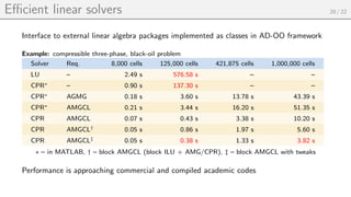
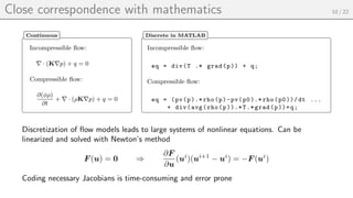
∇ · ∇(p + ρ~
g) = 0
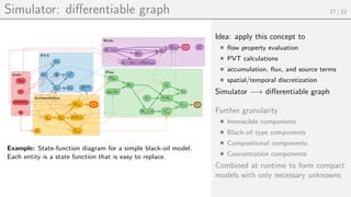
Oldest part of MRST:
Procedural programming
Structs for reservoir state, rock
parameters, wells, b.c., and source term
Fluid behavior: struct with function
pointers
Advantages:
hide specific details of geomodel and
fluid model
vectorization: efficient/compact code
unified access to key parameters

10. Rapid prototyping: discrete differentiation operators 9 / 22
Grid structure in MRST
5
6
7
8
2
1
2
3
4 1
3 4
5
6
7
8
9
c F(c)
1 1
1 2
1 3
1 4
2 5
2 6
2 7
2 8
2 2
3 1
.
.
.
.
.
.
.
.
.
.
.
.
Map: cell → faces
f
1
2
3
4
5
6
7
8
.
.
.
.
.
.
C1
3
1
1
9
4
2
2
2
.
.
.
.
.
.
C2
1
2
8
1
2
5
6
7
.
.
.
.
.
.
Map: face → cells
Idealized models Industry models

11. Rapid prototyping: discrete differentiation operators 9 / 22
Grid structure in MRST
5
6
7
8
2
1
2
3
4 1
3 4
5
6
7
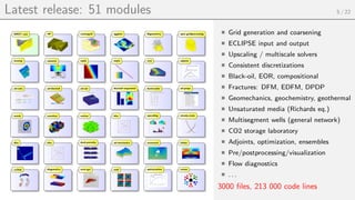
8
9
c F(c)
1 1
1 2
1 3
1 4
2 5
2 6
2 7
2 8
2 2
3 1
.
.
.
.
.
.
.
.
.
.
.
.
Map: cell → faces
f
1
2
3
4
5
6
7
8
.
.
.
.
.
.
C1
3
1
1
9
4
2
2
2
.
.
.
.
.
.
C2
1
2
8
1
2
5
6
7
.
.
.
.
.
.
Map: face → cells
Idealized models Industry models
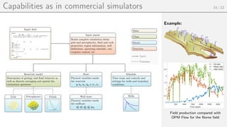
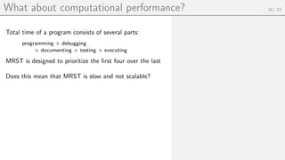
For finite volumes, discrete grad operator maps from cell pair C1(f), C2(f) to face f:
grad(p)[f] = p[C2(f)] − p[C1(f)],
where p[c] is a scalar quantity associated with cell c. Discrete div maps from faces to cells
Both are linear operators and can be represented as sparse matrix multiplications

12. Close correspondence with mathematics 10 / 22
Incompressible flow:
∇ · (K∇p) + q = 0
Compressible flow:
∂(φρ)
∂t
+ ∇ · (ρK∇p) + q = 0
Continuous
Incompressible flow:
eq = div(T .* grad(p)) + q;
Compressible flow:
eq = (pv(p).* rho(p)-pv(p0).* rho(p0))/dt ...
+ div(avg(rho(p)).*T.* grad(p))+q;
Discrete in MATLAB

13. Close correspondence with mathematics 10 / 22
Incompressible flow:
∇ · (K∇p) + q = 0
Compressible flow:
∂(φρ)
∂t
+ ∇ · (ρK∇p) + q = 0
Continuous
Incompressible flow:
eq = div(T .* grad(p)) + q;
Compressible flow:
eq = (pv(p).* rho(p)-pv(p0).* rho(p0))/dt ...
+ div(avg(rho(p)).*T.* grad(p))+q;
Discrete in MATLAB
Discretization of flow models leads to large systems of nonlinear equations. Can be
linearized and solved with Newton’s method
F (u) = 0 ⇒
∂F
∂u
(ui
)(ui+1
− ui
) = −F (ui
)
Coding necessary Jacobians is time-consuming and error prone

14. Automatic differentiation 11 / 22
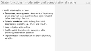
General idea:
Any code consists of a limited set of arithmetic operations and elementary functions
Introduce an extended pair, hx, 1i, i.e., the value x and its derivative 1
Use chain rule and elementary derivative rules to mechanically accumulate derivatives at
specific values of x
– Elementary: v = sin(x) −→ hvi = hsin x, cos xi
– Arithmetic: v = fg −→ hvi = hfg, fgx + fxgi
– Chain rule: v = exp(f(x)) −→ hvi = hexp(f(x)), exp(f(x))f0
(x)i
Use operator overloading to avoid messing up code
[x,y] = initVariablesADI(1,2);
z = 3*exp(-x*y)
x = ADI Properties:
val: 1
jac: {[1] [0]}
y = ADI Properties:
val: 2
jac: {[0] [1]}
z = ADI Properties:
val: 0.4060
jac: {[-0.8120] [-0.4060]}
∂x
∂x
∂x
∂y
∂y
∂x
∂y
∂y
∂z
∂x x=1,y=2
∂z
∂y x=1,y=2

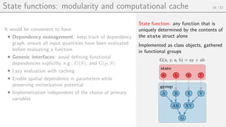
15. Example: incompressible single-phase flow 12 / 22
% Make grid
G = twister(cartGrid ([8 8]));
G = computeGeometry (G);
% Set source terms (flow SW -> NE)
q = zeros(G.cells.num ,1);
q([1 end ]) = [1 -1];
% Unit insotropic permeability
K = ones(G.cells.num ,4); K(: ,[2 3]) = 0;
% Make grid using external grid generator
pv = [-1 -1; 0 -.5; 1 -1; 1 1; 0 .5; -1 1; -1 -1];
fh = @(p,x) 0.025 + 0.375* sum(p.^2 ,2);
[p,t] = distmesh2d(@dpoly , fh , 0.025 , [-1 -1; 1 1], pv , pv);
G = computeGeometry (pebi( triangleGrid (p, t)));
% Set source terms (flow SW -> NE)
q = zeros(G.cells.num ,1);
v = sum(G.cells.centroids ,2);
[~,i1]= min(v); [~,i2]= max(v);
q([i1 i2]) = [1 -1];

16. Example: incompressible single-phase flow 12 / 22
% Make grid
G = twister(cartGrid ([8 8]));
G = computeGeometry (G);
% Set source terms (flow SW -> NE)
q = zeros(G.cells.num ,1);
q([1 end ]) = [1 -1];
% Unit insotropic permeability
K = ones(G.cells.num ,4); K(: ,[2 3]) = 0;
% Make grid using external grid generator
pv = [-1 -1; 0 -.5; 1 -1; 1 1; 0 .5; -1 1; -1 -1];
fh = @(p,x) 0.025 + 0.375* sum(p.^2 ,2);
[p,t] = distmesh2d(@dpoly , fh , 0.025 , [-1 -1; 1 1], pv , pv);
G = computeGeometry (pebi( triangleGrid (p, t)));
% Set source terms (flow SW -> NE)
q = zeros(G.cells.num ,1);
v = sum(G.cells.centroids ,2);
[~,i1]= min(v); [~,i2]= max(v);
q([i1 i2]) = [1 -1];
S = setupOperatorsTPFA(G,rock); % Define Div, Grad, etc
p = initVariablesADI(zeros(G.cells.num,1)); % Initialize p as AD variable
eq = S.Div(S.T .∗ S.Grad(p)) + q; % Residual equation: F = Ap + q
eq(1) = eq(1) + p(1); % Fixate pressure
p =−eq.jac{1}eq.val; % Solve system A

17. Example: compressible two-phase flow 13 / 22
[p, sW] = initVariablesADI(p0, sW0); % Primary variables
[pIx, sIx] = deal(1:nc, (nc+1):(2∗nc)); % Indices of p/S in eq. system
[tol, maxits] = deal(1e−5, 15); % Iteration control
t = 0;
while t < totTime,
t = t + dt;
resNorm = 1e99; nit=0;
[p0, sW0] = deal(value(p), value(sW)); % Prev. time step not AD variable
while (resNorm > tol) &
& (nit<= maxits) % Nonlinear iteration loop
% one Newton iteration
end
if nit > maxits,
error('Newton solves did not converge')
end
end
% Evaluate equations
[rW, rO, vol] = deal(rhoW(p), rhoO(p), pv(p)));
:
water = (vol.∗rW.∗sW − vol0.∗rW0.∗sW0)./dt + div(vW);
water(inIx) = water(inIx) − inRate.∗rhoWS;
:
eqs = {oil, water}; % concatenate equations
eq = cat(eqs{:}); % assemble
res = eq.val; % residual
upd =−(eq.jac{1} res); % Newton update
% Update variables
p.val = p.val + upd(pIx);
sW.val = sW.val + upd(sIx);
sW.val = max( min(sW.val, 1), 0);
resNorm = norm(res);
nit = nit + 1; ∂W
∂p
∂O
∂p
∂W
∂Sw
∂O
∂Sw

18. The AD-OO simulator framework 14 / 22
Primary vars
[Res, Jac], info
Assemble: Ax = b
δx
Update variables:
p ← p + δp, s ← s + δs, ...
Initial ministep:
∆t
Adjusted:
∆t̃
Write to storage
3D visualization
Well curves
State(Ti), ∆Ti, Controls(Ci)
State(Ti + ∆Ti)
Type color legend
Class
Struct
Function(s)
Input
Contains object
Optional output
Initial state Physical model
Schedule
Steps
Time step and control numbers
{(∆T1, C1), ..., (∆Tn, Cn)},
Controls
Different wells and bc
{(W1, BC1), ..., (Wm, BCm)}
Simulator
Solves simulation schedule comprised
of time steps and drive mechanisms
(wells/bc)
simulateScheduleAD
Nonlinear solver
Solves nonlinear problems sub-divided
into one or more mini steps using
Newton’s method
Time step selector
Determines optimal time steps
SimpleTimeStepSelector,
IterationCountSelector,
StateChangeTimeStepSelector, ...
Result handler
Stores and retrieves simulation data
from memory/disk in a transparent
and efficient manner.
Visualization
Visualize well curves, reservoir proper-
ties, etc
plotCellData, plotToolbar,
plotWellSols, ...
State
Primary variables: p, sw, sg, Rs, Rv...
Well solutions
Well data: qW, qO, qG, bhp, ...
Physical model
Defines mathematical model: Resid-
ual equations, Jacobians, limits on
updates, convergence definition...
TwoPhaseOilWaterModel,
ThreePhaseBlackOilModel
Well model
Well equations, control switch, well-
bore pressure drop, ...
Linearized problem
Jacobians, residual equations and
meta-information about their types
Linear solver
Solves linearized problem and returns
increments
BackslashSolverAD, AGMGSolverAD,
CPRSolverAD, MultiscaleSolverAD, ...

19. Capabilities as in commercial simulators 15 / 22
Data
Class
Struct
Function
Input
Contains
Input deck
Input parser
Reads complete simulation decks:
grid and petrophysics, fluid and rock
properties, region information, well
definitions, operating schedule, con-
vergence control, etc
Reservoir model
Description of geology and fluid behavior as
well as discrete averaging and spatial dis-
cretization operators
Petrophysics
Grid Fluids
0 0.2 0.4 0.6 0.8 1
0
0.2
0.4
0.6
0.8
1
State
Physical variables inside
the reservoir
p, sw, so, sg, c, rv, rs
Well state
Physical variables inside
the wellbore
qs
w, qs
o, qs
g, qs
p, pbh
Schedule
Time steps and controls and
settings for wells and boundary
conditions
Wells
Example:
500 1000 1500 2000 2500 3000
Time (days)
0
0.5
1
1.5
2
2.5
Oil (stb)
Water (stb)
Gas (mscf)
Field production compared with
OPM Flow for the Norne field

20. State functions: modularity and computational cache 16 / 22
It would be convenient to have:
Dependency management: keep track of dependency
graph, ensure all input quantities have been evaluated
before evaluating a function
Generic interfaces: avoid defining functional
dependencies explicitly, e.g., G(S), and G(p, S).
Lazy evaluation with caching
Enable spatial dependence in parameters while
preserving vectorization potential
Implementation independent of the choice of primary
variables

21. State functions: modularity and computational cache 16 / 22
It would be convenient to have:
Dependency management: keep track of dependency
graph, ensure all input quantities have been evaluated
before evaluating a function
Generic interfaces: avoid defining functional
dependencies explicitly, e.g., G(S), and G(p, S).
Lazy evaluation with caching
Enable spatial dependence in parameters while
preserving vectorization potential
Implementation independent of the choice of primary
variables
State function: any function that is
uniquely determined by the contents of
the state struct alone
Implemented as class objects, gathered
in functional groups
A B X Y
AB XY
G
group
a b x y
state
G(x, y, a, b) = xy + ab

22. Simulator: differentiable graph 17 / 22
Vi,α Vi
λf
i,α
gρα∆z
Tf Θα
vα
Θα
Θα ≤ 0
∇pα
Tf
λf
α
Flux
Qi,α Qi
W → c
ρw
α
pc − pbh − g∆zρmix
qα
WI
Wells
ρα
pα Φ wp
i
bα
µα
Rmax
s
PVT
pc λi,α
ραxi,α
Mi,α Mi
λα
kα
Accumulation
bhp
rs
pressure
s
state
Example: State-function diagram for a simple black-oil model.
Each entity is a state function that is easy to replace.
Idea: apply this concept to
flow property evaluation
PVT calculations
accumulation, flux, and source terms
spatial/temporal discretization
Simulator −→ differentiable graph
Further granularity
Immiscible components
Black-oil type components
Compositional components
Concentration components
Combined at runtime to form compact
models with only necessary unknowns

23. What about computational performance? 18 / 22
Total time of a program consists of several parts:
programming + debugging
+ documenting + testing + executing
MRST is designed to prioritize the first four over the last
Does this mean that MRST is slow and not scalable?

24. What about computational performance? 18 / 22
Total time of a program consists of several parts:
programming + debugging
+ documenting + testing + executing
MRST is designed to prioritize the first four over the last
Does this mean that MRST is slow and not scalable?
No, I would say its is surprisingly efficient
Potential concerns:
MATLAB is interpreted
cure: JIT, vectorization, logical indexing,
pre-allocation, highly-efficient libraries
Redundant computations
cure: state functions = dependency
graph + computational cache
Computational overhead
cure: new auto diff backends
Scalability/performance
cure: external high-end iterative solvers

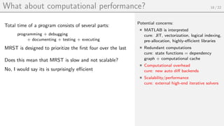
25. New backends for automatic differentiation 19 / 22
1 104
1 105
1 106
2 106
Number of cells
10-2
100
102
Assembly
time
[s]
single-phase
3ph, immiscible
3ph, blackoil
6c, compositional
0.5 s / million cells
50 s / million cells
overhead dominates
New AD backends: storage optimized wrt access pattern, MEX-accelerated operations

26. Efficient linear solvers 20 / 22
Interface to external linear algebra packages implemented as classes in AD-OO framework
Example: compressible three-phase, black-oil problem
Solver Req. 8,000 cells 125,000 cells 421,875 cells 1,000,000 cells
LU – 2.49 s 576.58 s – –
CPR∗
– 0.90 s 137.30 s – –
CPR∗
AGMG 0.18 s 3.60 s 13.78 s 43.39 s
CPR∗
AMGCL 0.21 s 3.44 s 16.20 s 51.35 s
CPR AMGCL 0.07 s 0.43 s 3.38 s 10.20 s
CPR AMGCL†
0.05 s 0.86 s 1.97 s 5.60 s
CPR AMGCL‡
0.05 s 0.38 s 1.33 s 3.82 s
∗ – in MATLAB, † – block AMGCL (block ILU + AMG/CPR), ‡ – block AMGCL with tweaks
Performance is approaching commercial and compiled academic codes

27. New book: Advanced modelling with MRST 21 / 22
Berge et al.: Constrained Voronoi grids Al Kobaisi & Zhang: nonlinear FVM Lie & Møyner: multiscale methods
Wong et al.: embedded discrete fractures Olorode et al.; fractured unconventionals March et al.: unified framework, fractures
Varela et al.: unsaturated poroelasticity Collignon et al.: geothermal systems Andersen: coupled flow & geomechanics
Møyner: compositional
Sun et al.: chemical EOR
Møyner: state functions, AD backends
Klemetsdal & Lie: discontinuous Galerkin

28. Acknowledgements 22 / 22
Thanks to all my co-developers at SINTEF (Olav Møyner,
in particular), our master and PhD students, and our
national and international collaborators.
Thanks also to all MRST users who have asked interesting
questions that have helped us shape the software
Funding:
Research Council of Norway
SINTEF
Equinor: gold open access for the
MRST textbook
Chevron, Ecopetrol, Eni, Equinor,
ExxonMobil, Shell, SLB, Total,
Wintershall DEA, . . .