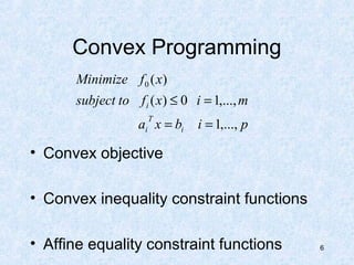
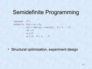
The document discusses CVXOPT, a Python-based suite for convex optimization that offers various solvers for different types of programming problems, including linear, quadratic, and semidefinite programming. It explains the key concepts of convex sets and functions, outlines the structure of solvers like conelp and coneqp, and provides examples of applications in areas such as finance and structural optimization. The presentation ultimately highlights the software's capabilities and potential customization options for improved performance.

1. CVXOPT:
A Python Based Convex
Optimization Suite
11 May 2012
Industrial Engineering Seminar
Andrew B. Martin

2. Easy and Hard
• Easy Problems - efficient and reliable
solution algorithms exist
• Once distinction was between
Linear/Nonlinear, now
Convex/Nonconvex
2

3. Outline
• What is CVXOPT?
• How does CVXOPT solve problems?
• What are some interesting applications
of CVXOPT?
3

4. Convex Sets
• For any x,y
belonging to the set
C, the chord
connecting x and y
is contained within
C.
4

5. Convex Functions
• A real valued
function mapping a
set X to R where X
is a convex set and
for any x, y
belonging to X
f (tx + (1 − t ) y ) ≤ tf ( x) + (1 − t ) f ( y )
0 ≤ t ≤1
5

6. Convex Programming
Minimize f 0 ( x)
subject to f i ( x) ≤ 0 i = 1,..., m
T
ai x = bi
i = 1,..., p
• Convex objective
• Convex inequality constraint functions
• Affine equality constraint functions
6

7. Linear Programming
• Supply Chain Modeling (Forestry)
7

8. Quadratic Programming
• Least Squares and Constrained Least
Squares
• Quantitative Finance
8

9. Second Order Cone
Programming
• Robust Linear Programming
• Truss design, robotic grasping force, antenna
design
9

10. Example: Robust LP
Minimize cT x
subject to aiT x ≤ bi ∀ai ∈ Ε i i = 1,..., m
_
Ei = {a i + Pi u | u 2 ≤ 1} Pi ∈ ℜ nxn
sup{aiT x | ai ∈ Ε i } ≤ bi
_T
sup{aiT x | ai ∈ Ε i } = a i x + Pi T x
2
Minimize cT x
_T
subject to a x + Pi T x ≤ bi i = 1,..., m
2
10

11. Semidefinite Programming
• Structural optimization, experiment design
11

12. Geometric Programming
Minimize
f 0 ( x)
Subject to
f i ( x) ≤ 1 i = 1,..., n
h j ( x) = 1 j = 1,..., m
• Posynomial objective and inequality
constraint functions.
• Monomial equality constraint functions
12

13. Globally Optimal Points
• Any locally optimal point is globally
optimal!
• No concern of getting stuck at
suboptimal minimums.

14. Overview CVXOPT
• Created by L. Vandenberghe and
J. Dahl of UCLA
• Extends pythons standard libraries
– Objects matrix and spmatrix
• Defines new modules e.g. BLAS,
LAPACK, modeling and solvers
14

15. cvxopt.solvers
•
•
•
•
Cone solvers: conelp, coneqp
Smooth nonlinear solvers: cp, cpl
Geometric Program solver: gp
Customizable: kktsolver
15

16. Cone Programs
• s belongs to C, the Cartesian product of a
nonnegative orthant, a number of second
order cones and a number of positive
semidefinite cones
16

17. Cone Solvers
• Apply Primal-Dual Path following
Interior Point algorithms with NesterovTodd Scaling to the previous problem
• Specify cone dimension with variable
dims
• Separate QP and LP solvers
17

18. solvers.coneqp
• coneqp(P, q, G, h, A, b, dims, kktsolver)
• Linearize Central Path Equations
(Newton Equations)
• Solving these is the most expensive step
• Transform N.E. into KKT system
18

19. solvers.coneqp
Central Path Equations
0   P
0  +  A
  
 s  G
  
G T   x  − c 
   
0   y  =  b , ( s, z )  0, z = − µg ( s )
0  z   h 
   
AT
0
0
Newton Equations
P

A
G

AT
0
0
  x  a 
   
0   y  = b 
− W TW   z   c 
   
GT
19

20. solvers.coneqp
KKT System
 P

 A
W −T G

T
A
0
0
T
G W
0
−I
−1
 x   a 
  
y = b 


 Wz  W −T c 

  
20

21. Constrained Regression
21

22. >> from cvxopt import matrix, solvers
>> A = matrix([ [ .3, -.4, -.2, -.4, 1.3 ], [ .6, 1.2, -1.7, .3, -.3 ], /
-.3, .0, .6, -1.2, -2.0 ] ])
>> b = matrix([ 1.5, .0, -1.2, -.7, .0])
>> m, n = A.size
>>> I = matrix(0.0, (n,n))
>> I[::n+1] = 1.0
>> G = matrix([-I, matrix(0.0, (1,n)), I])
>> h = matrix(n*[0.0] + [1.0] + n*[0.0])
>> dims = {'l': n, 'q': [n+1], 's': []}
>> x = solvers.coneqp(A.T*A, -A.T*b, G, h, dims)['x']
>> print(x)
7.26e-01]
6.18e-01]
3.03e-01]
22

23. solvers.conelp
• Coneqp demands strict primal-dual
feasibility. Conelp can detect
infeasibility.
• Embeds primal and dual LPs into one
LP
• Algorithm similar to coneqp except two
QR factorizations used to solve KKT
System
23

24. solvers.conelp
Self-dual Cone LP
Minimize 0
0  0
0 
  = − A
s −G
   T
κ  − c

AT
0
0
− bT
GT
0
0
− hT
C x
 
b  y
, ( s, κ , z ,τ )  0
h  z 
 
0  τ 

24

25. dims = {'l': 2, 'q': [4, 4], 's': [3]}
25

26. Nonlinear Solvers
• Solvers.cpl for linear objective problems
• User specifies F function to evaluate
gradients and hessian of constraints
• Solvers.cpl(F, G, h, A, b, kktsolver)
26

27. solvers.cpl
KKT System

H
A
~
G

T
A
0
0
m

G  u x  bx 
0  u y  = by ,
   
− W T W  u z  bz 
   

~
T
~
H = ∑ z k ∇ f k ( x), G = [∇f1 ( x) ... ∇f m ( x) G T ]T
2
k =0
27

28. solvers.cp
• For problems with a nonlinear objective
function
• Problem transformed into epigraph form and
solvers.cpl algorithm applied
28

29. solvers.cp
Robust Least Squares
from cvxopt import solvers, matrix, spdiag, sqrt, div
def robls(A, b, rho) :
m, n = A.size
def F(x = None, z = None) :
if x is None : return 0, matrix(0.0, (n,1))
y = A*x -b
w = sqrt(rho + y * *2)
f = sum(w)
Df = div(y, w).T * A
if z is None : return f, Df
H = A.T * spdiag(z[0] * rho * (w * * - 3)) * A
return f, Df, H
Minimize
m
∑ φ((Ax-b) )
k =1
k
where φ (u ) = ρ + u 2
return solvers.cp(F)[' x' ]
29

30. Geometric Solver
• GP transformed to equivalent convex form
and solvers.cp is applied
• Solvers.gp(F, G, h, A, b)
30

31. Exploiting Structure
• None of the previously mentioned
solvers take advantage of problem
structure
• User specified kktsolvers and python
functions allow for customization
• Potential for better than commercial
software performance
31

32. Exploiting Structure
M
N
CVXOPT
CVXOPT/BLAS
MOSEK 1.15
MOSEK 1.17
500
100
0.12
0.06
0.75
0.40
1000 100
0.22
0.11
1.53
0.81
1000 200
0.52
0.25
1.95
1.06
2000 200
1.23
0.60
3.87
2.19
1000 500
2.44
1.32
3.63
2.38
2000 500
5.00
2.68
7.44
5.11
2000 1000
17.1
9.52
32.4
12.8
•
L1-norm approximation solution times for six randomly
generated problems of dimension mxn (ref)
32

33. Interlude: iPython
• Interactive Programming Environment
• explore algorithms, and perform data
analysis and visualization.
• It facilitates experimentation - new ideas
can be tested on the fly
33

34. iPython - Features
• Magic Commands - e.g. %run
• Detailed Exception Traceback
• OS Shell Commands
• Extensive GUI support
34

35. Facility Layout Problem
• As Nonlinearly Constrained Program
• As Geometric Program
• As Quadratic Program
35

36. Nonlinearly Constrained
Facility Layout Problem
Minimize W + H
Subject to wk hk ≤ Areamin
x k + wk ≤ x j
x k + wk ≤ W
yk + hk ≤ y j
yk + hk ≤ H
1 / α ≤ wk / hk ≤ α
36

37. 200 Modules

38. Geometric Program
Minimize W * H
Subject to x j * xi−1 + w j * xi−1 ≤ 1
x j *W −1 + w j *W −1 ≤ 1
y j * yi−1 + h j * yi−1 ≤ 1
y j * H −1 + h j * H −1 ≤ 1
Areamin * w−1 * h −1 ≤ 1
j
j
1 / α ≤ w j * h −1 ≤ α
j
38

39. Quadratic Program
Minimize
∑∑
i
j
xi − x j
flowi , j *
yi − y j
2
+ β (W + H )
2
subject to x j + w j ≤ xi
x j + wj ≤ W
y j + h j ≤ yi
y j + hj ≤ H
− w j ≤ − Areamin
− h j ≤ − Areamin
1/ α ≤ wj / hj ≤ α
39

40. 65 Modules

41. Closing
• CVXOPT: Software for Convex
Optimization
• How will you use it?
• andrew.b.martin@dal.ca
41

42. References
42