The document discusses the acceleration of pseudo-marginal Markov Chain Monte Carlo (MCMC) methods using Gaussian processes in the context of Bayesian statistics. It presents various algorithms and techniques for improving the efficiency and scalability of these methods, focusing on the Bayesian indirect likelihood and adaptive algorithms. Key components include the utilization of auxiliary models and the optimization of computational resources through parallel precomputation.

1. Accelerating Pseudo-Marginal MCMC
using Gaussian Processes
Matt Moores
joint work with Chris Drovandi (QUT) and Richard Boys (Newcastle)
October 28, 2016
Matt Moores Algorithms Seminar October 28, 2016 1 / 10

2. Grouped independence Metropolis-Hastings (GIMH)
Auxiliary variable algorithms (pseudo-marginal, exchange, ABC)
have two main components:
1 Primary chain targets the posterior π(θ | y)
2 Auxiliary chain constructs unbiased, non-negative estimates of the
intractable likelihood ˆp(y | θ)
Algorithm 1 GIMH
Input: θ(t−1) ∈ Θ, φ
(t−1)
N = ˆp(y | θ(t−1))
1: Propose θ ∼ q(· | θ(t−1))
2: Simulate x1, . . . , xN
iid
∼ q(x)
3: Estimate φN = 1
N
N
i=1
p(y|xi,θ )p(xi|θ )
q(xi)
4: Calculate α = 1 ∧
φN p(θ ) q(θ(t−1)|θ )
φt−1 p(θt−1) q(θ |θt−1)
Output: return (θ , φN) with probability α, else return (θ(t−1), φ
(t−1)
N )
Matt Moores Algorithms Seminar October 28, 2016 2 / 10
Beaumont (Genetics, 2003)
Andrieu & Roberts (Ann. Stat., 2009)

3. Bayesian indirect likelihood (BIL)
Construct an auxiliary model, ˆpBIL(y | ψ(θ))
Reuse previous values of φ
(t)
N (or auxiliary variables x1, . . . , xN)
Enable local adaptation of q(· | θ) (Sejdinovic et al., 2014)
Optional precomputation step:
Utilise massively parallel hardware to simulate from q(x)
Explore parameter space Θ more efficiently:
Monte Carlo within Metropolis (MCWM)
Wang-Landau
(Bornn et al., 2013; Jacob & Ryder, 2014)
Bayesian optimisation
(Gutmann & Corander, 2016)
Locate region of high posterior support (Wilkinson, 2014)
Can then invert ˆpBIL(y | ψ(θ)) to initialise the primary chain with a
“warm start.”
Matt Moores Algorithms Seminar October 28, 2016 3 / 10
Drovandi, Pettitt & Lee (Statist. Sci., 2015)

4. Which auxiliary model to use?
Importance sampling
(Liang, Jin, Song & Liu, 2016)
Piecewise linear
(Moores, Drovandi, Mengersen & Robert, 2015)
k-nearest neighbour
(Sherlock, Golightly & Henderson, 2015)
Gaussian process (GP)
(Wilkinson, 2014; Meeds & Welling, 2014; Järvenpää et al., 2016)
Local polynomials or GP with compact support
(Conrad, Marzouk, Pillai & Smith, 2016)
Kernel methods
(Sejdinovic et al., 2014; Strathmann et al., 2015)
Matt Moores Algorithms Seminar October 28, 2016 4 / 10

5. Gaussian Processes (GPs)
Multivariate normal with mean function m(θ) and covariance c(θ, θ ):
− log {p(y | θ)} ∼ N m(θ), c(θ, θ ) (1)
Under certain assumptions:
π(θ | y) is a compact Hilbert space with finite dimension, d
Boundary ∂π(θ | y) satisfies the cone condition
c(θ, θ ) is a squared exponential or Matérn covariance
Training points θ1, . . . , θJ ∈ Θ are on a regular lattice
a GP is a consistent approximation to the negative log-likelihood
(Stuart & Teckentrup, 2016)
Can use output of precomp. step to test assumptions empirically
(Ratmann et al. 2013) or for Bayesian model choice (Järvenpää et al.
2016)
Matt Moores Algorithms Seminar October 28, 2016 5 / 10

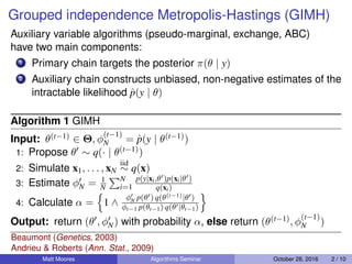
6. Multiplicative Noise
Can’t evaluate p(y|θ) pointwise, but by lognormal CLT:
φ
(t)
N = W p y | θ(t)
(2)
E[W] = 1 (3)
log{W}
d
−−−−→
N→∞
N −
1
2
σ2
, σ2
(4)
when x1, . . . , xN are generated from a particle filter
(Bérard, Del Moral & Doucet, 2014)
We can account for this noise by adding a nugget term to our GP:
− log ˆφ
(j)
N ∼ N mβ(θ) +
δ
2
, cγ(θ, θ ) + δI (5)
where θ(j), φ
(j)
N
J
j=1
are obtained from the precomputation step
Matt Moores Algorithms Seminar October 28, 2016 6 / 10

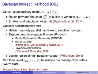
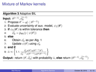
7. Delayed Acceptance (DA)
Algorithm 2 BIL with DA
Input: θ(t−1) ∈ Θ, φ
(t−1)
N = ˆp(y | θ(t−1))
1: Propose θ ∼ q(· | θ(t−1))
2: Calculate αBIL = 1 ∧ ˆpBIL(y|ψ(θ )) p(θ ) q(θ(t−1)|θ )
ˆpBIL(y|ψ(θ(t−1))) p(θ(t−1)) q(θ |θ(t−1))
Output: return (θ(t−1), φ
(t−1)
N ) with probability 1 − α, else
3: Obtain φN as per Alg. 1
4: Calculate αDA = 1 ∧
φN ˆpBIL(y|ψ(θ(t−1)))
φ
(t−1)
N ˆpBIL(y|ψ(θ ))
Output: return (θ , φN) with probability αDA, else return (θ(t−1), φ
(t−1)
N )
Matt Moores Algorithms Seminar October 28, 2016 7 / 10
Christen & Fox (JCGS, 2005)
Sherlock, Golightly & Henderson (arXiv:1509.00172 [stat.CO])

8. Mixture of Markov kernels
Algorithm 3 Adaptive BIL
Input: θ(t−1), ˆφ
(t−1)
N
1: Propose θ ∼ q(· | θ(t−1))
2: Evaluate uncertainty of aux. model, ψΣ(θ )
3: if ψΣ(θ ) is within tolerance then
4: ˆφN = ˆpBIL(y | ψ(θ ))
5: else
6: Obtain φN as per Alg. 1
7: Update ψ(θ ) using φN
8: end if
9: ˆα ≈ 1 ∧
ˆφN p(θ ) q(θ(t−1)|θ )
ˆφ
(t−1)
N p(θ(t−1)) q(θ |θ(t−1))
Output: return (θ , ˆφN) with probability ˆα, else return (θ(t−1), ˆφ
(t−1)
N )
Matt Moores Algorithms Seminar October 28, 2016 8 / 10

9. Summary
BIL can improve elapsed runtime and scalability of
pseudo-marginal methods:
Extrapolate between previous estimates of ˆp(y|θ)
Parallel precomputation step
DA preserves the exact posterior
Threshold for ψΣ(θ ) enables tradeoff between
accuracy and computational cost
Matt Moores Algorithms Seminar October 28, 2016 9 / 10

10. For Further Reading
C. C. Drovandi, M. Moores & R. Boys
Accelerating Pseudo-Marginal MCMC using Gaussian Processes.
Tech. Rep., QLD Univ. of Tech., 2015.
M. Moores, C. C. Drovandi, K. Mengersen & C. P. Robert
Pre-processing for approximate Bayesian computation in image analysis.
Statistics & Computing 25(1): 23–33, 2015.
C. C. Drovandi, A. N. Pettitt & A. Lee
Bayesian indirect inference using a parametric auxiliary model.
Statist. Sci. 30(1): 72–95, 2015.
M. Moores, A. N. Pettitt & K. Mengersen
Scalable Bayesian inference for the inverse temperature of a hidden Potts model.
arXiv:1503.08066 [stat.CO], 2015.
C. C. Drovandi, A. N. Pettitt & M. J. Faddy
Approximate Bayesian computation using indirect inference.
J. R. Stat. Soc. Ser. C 60(3): 317–337, 2011.
Matt Moores Algorithms Seminar October 28, 2016 10 / 10