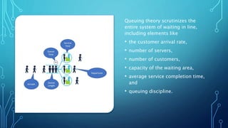
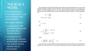
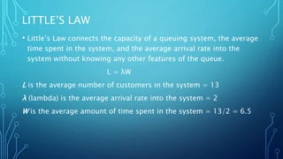
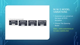
Queuing theory is the mathematical study of waiting lines, analyzing elements like arrival rates, number of servers, and service times. Introduced by Agner Krarup Erlang in the early 20th century, it provides insights into optimizing service efficiency. Key models, such as the M/M/s model, are utilized to understand customer behavior and system performance.

1. QUEUING THEORY
MUFADDAL HAIDERMOTA

2. WHAT ?
• Queuing theory (or queueing theory)
refers to the mathematical study of the
formation, function, and congestion of
waiting lines, or queues.
• At its core, a queuing situation involves
two parts :
1. Someone or something that
requests a service - usually referred to
as the customer, job, or request.
2. Someone or something that
completes or delivers the services -
usually referred to as the server.

3. Queuing theory scrutinizes the
entire system of waiting in line,
including elements like
• the customer arrival rate,
• number of servers,
• number of customers,
• capacity of the waiting area,
• average service completion time,
and
• queuing discipline.

4. HISTORY
• Introduced in the 20th century by Danish mathematician and engineer Agner
Krarup Erlang
• He worked for the Copenhagen Telephone Exchange and wanted to analyze
and optimize its operations.
• His mathematical analysis culminated in his 1920 paper “Telephone Waiting
Times”, which served as the foundation of applied queuing theory. The
international unit of telephone traffic is called the Erlang in his honor.

5. DESIGN
CONSIDERATI
ON
In designing queueing systems we need to aim for a balance
between service to customers (short queues implying many
servers) and economic considerations (not too many servers).
In essence all queuing systems can be broken down into
individual sub-systems consisting of entities queuing for
some activity (as shown below).
Typically we can talk of this individual sub-system as dealing
with customers queuing for service.

6. To analyze this sub-system we need information relating to :
• Arrival Process – batch or bulk, interarrival time distribution
• Service Mechanism – resources, service time distribution, no.of
servers, server arrangement (series or parallel),
preemption allowed or not.
• Queue Characteristics – opt for a queue discipline to follow, do
we have:
 balking (customers deciding not to join the queue if it is too long)
 reneging (customers leave the queue if they have waited too long for
service)
 jockeying (customers switch between queues if they think they will get
served faster by so doing)
 a queue of finite capacity or (effectively) of infinite capacity

7. KENDALL’S NOTATION
• λ: the mean arrival rate : number of arrivals per unit time
• μ: the mean service rate : number of customers served per unit time
• A: the arrival process probability distribution. (inter-arrival time
distribution)
• B: the service process probability distribution. (service time
distribution)
• C: the number of servers.
• D: the maximum number of customers allowed in the system at any
given time, waiting or being served (without getting bumped)
• E: maximum number of customers in total
• F: Queuing discipline that is followed

8. • Shorthand notation of the
type A/B/C/D/E/F
• The simplest member of queue
model is M/M/1/∞/∞/FCFS.
• This means that we have a single
server; the service rate
distribution is exponential;
arrival rate distribution is
poisson process; with infinite
queue length allowed and
anyone allowed in the system;
finally its a first come first
served model.
Possible values of A
Possible values of B

9. POISSON PROCESS
• Poisson Process is a model for a
series of discrete event where the
average time between the events is
known, but the exact timing of the
event is random.
• The most common assumption is that
they follow a Poisson Process.
At a given time period the
number of arrivals follow a
Poisson distribution.
Another way to characterize this
process is that the interarrival
time (time between two
consecutive arrivals) follows an
exponential distribution.
N(t) is the number of arrivals during a time
period of duration t and N(t) has a Poisson

10. POISSON PROCESS CONTD…
The defining properties of this process that is considered while
applying to a specific service system are:
• Customers arrive one at a time.
• The probability that a customer arrives at any time is independent of
when other customers arrived.
• The probability that a customer arrives at a given time is independent
of the time.
• The average rate (events per time period) is constant.
• Two events cannot occur at the same time.

11. THE M/M/S
MODEL
The M/M/s model or
Erlang delay model is the
most commonly used
queuing model.
This model assumes :
• a single queue with
unlimited waiting room
that feeds into s
identical servers.
• Customers arrive
according to a Poisson
process with a constant
rate, and the service
duration has an
exponential

12. LITTLE’S LAW
• Little’s Law connects the capacity of a queuing system, the average
time spent in the system, and the average arrival rate into the
system without knowing any other features of the queue.
L = λW
L is the average number of customers in the system = 13
λ (lambda) is the average arrival rate into the system = 2
W is the average amount of time spent in the system = 13/2 = 6.5

13. BRINGING IT
ALL
TOGETHER

14. M/M/S MODEL
VARIATIONS
• Customers are served on
the basis of FCFS
discipline
• Choose The Queuing
Model
https://www.supositorio.co
m/rcalc/rcalclite.htm

15. QUEUE PSYCHOLOGY
• Queuing theory is helpful in
explaining the math behind how
queues run. But when queues
involve humans, queue psychology
is important to understand the
queue experience as well.
• Queue psychology research shows
it’s not the length of the wait that
determines how positive or negative
the queue experience is, but rather
how people feel while waiting.

16. REFRENCES
• http://people.brunel.ac.uk/~mastjjb/jeb/or/queue.html
• https://queue-it.com/blog/queuing-theory/
• https://www0.gsb.columbia.edu/mygsb/faculty/research/pubfi
les/5474/queueing%20theory%20and%20modeling.pdf
• https://www.analyticsvidhya.com/blog/2016/04/predict-
waiting-time-queuing-theory/
• https://towardsdatascience.com/the-poisson-distribution-
and-poisson-process-explained-4e2cb17d459

17. THANK YOU