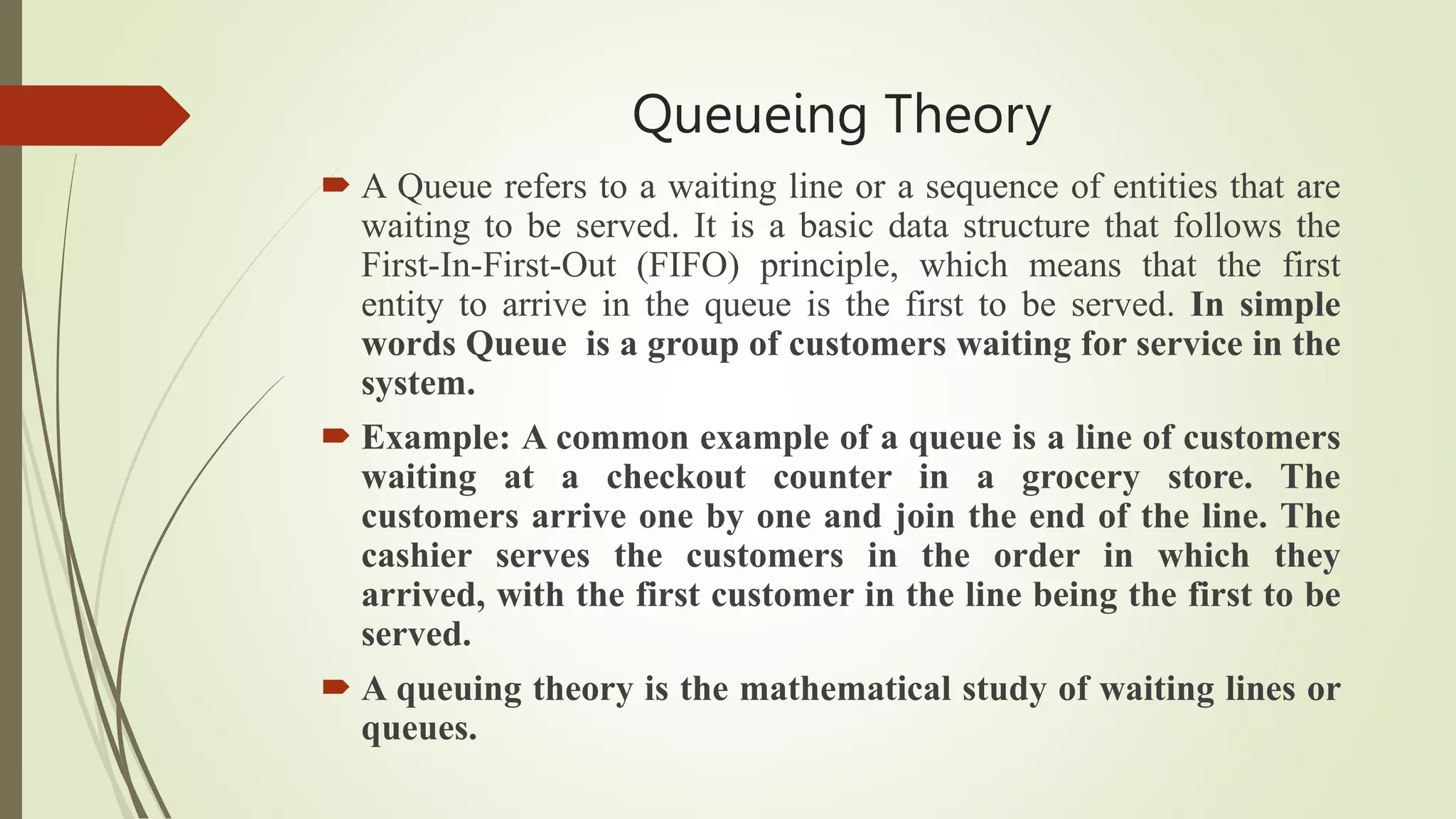
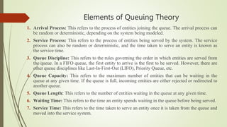
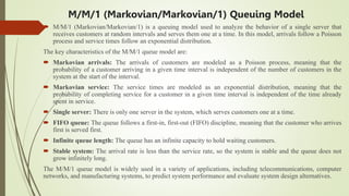
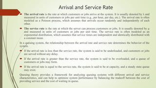
Queueing theory is the mathematical study of waiting lines or queues. A queue refers to a sequence of entities waiting to be served based on the first-in-first-out (FIFO) principle. Common examples include lines at checkout counters. Key elements of queueing theory include the arrival and service processes, queue discipline, capacity, length, waiting time, and service time. The M/M/1 queue model analyzes a single server queue where arrivals and services times follow Markovian processes. It is used to predict performance and evaluate system design.

1. Queueing Theory
 A Queue refers to a waiting line or a sequence of entities that are
waiting to be served. It is a basic data structure that follows the
First-In-First-Out (FIFO) principle, which means that the first
entity to arrive in the queue is the first to be served. In simple
words Queue is a group of customers waiting for service in the
system.
 Example: A common example of a queue is a line of customers
waiting at a checkout counter in a grocery store. The
customers arrive one by one and join the end of the line. The
cashier serves the customers in the order in which they
arrived, with the first customer in the line being the first to be
served.
 A queuing theory is the mathematical study of waiting lines or
queues.

2. Elements of Queuing Theory
1. Arrival Process: This refers to the process of entities joining the queue. The arrival process can
be random or deterministic, depending on the system being modeled.
2. Service Process: This refers to the process of entities being served by the system. The service
process can also be random or deterministic, and the time taken to serve an entity is known as
the service time.
3. Queue Discipline: This refers to the rules governing the order in which entities are served from
the queue. In a FIFO queue, the first entity to arrive is the first to be served. However, there are
other queue disciplines like Last-In-First-Out (LIFO), Priority Queue, etc.
4. Queue Capacity: This refers to the maximum number of entities that can be waiting in the
queue at any given time. If the queue is full, incoming entities are either rejected or redirected to
another queue.
5. Queue Length: This refers to the number of entities waiting in the queue at any given time.
6. Waiting Time: This refers to the time an entity spends waiting in the queue before being served.
7. Service Time: This refers to the time taken to serve an entity once it is taken from the queue and
moved into the service system.

3. Queue Discipline
Queue discipline refers to the set of rules or
algorithms used to determine the order in which
entities are served from a queue.
It is an important aspect of queueing theory and
plays a crucial role in determining the performance
of a queueing system.
The choice of queue discipline depends on the
nature of the system being modeled and the
objectives of the queueing system.

4. Types of Queue Discipline
 First-In-First-Out (FIFO): In this discipline, the first entity to arrive in the queue is
the first to be served. It follows the principle of "first come, first served." This is the
most common queue discipline used in real-world situations.
 Last-In-First-Out (LIFO): In this discipline, the last entity to arrive in the queue is
the first to be served. It is also known as the "stack" or "pushdown" discipline.
 Priority Queue: In this discipline, entities are served according to their priority
level. The entities with higher priority are served before those with lower priority.
 Shortest Job First (SJF): In this discipline, entities are served based on their
service time. The entity with the shortest service time is served first.
 Priority and Shortest Job First (PSJF): In this discipline, entities are served based
on both their priority level and service time.
 Round Robin: In this discipline, entities are served in a cyclic order. Each entity is
served for a fixed time slice, and if it is not completed within the time slice, it is
preempted and added back to the end of the queue.

5. Assumptions of Queuing model
1. Arrival Process: The arrival process of entities to the queue is assumed to follow a probabilistic
distribution, such as Poisson or exponential distribution. This means that the arrival of entities is
random and unpredictable.
2. Service Process: The service time of entities is also assumed to follow a probabilistic distribution.
This means that the time taken to serve an entity is random and can vary from one entity to another.
3. Queue Discipline: The queue is assumed to follow a specific discipline, such as First-In-First-Out
(FIFO) or Priority Queue. The discipline is assumed to be fixed and not affected by external factors.
4. Queue Capacity: The queue is assumed to have a finite capacity, and once it reaches its capacity,
incoming entities are either rejected or redirected to another queue.
5. Service Rate: The rate at which entities are served is assumed to be constant and fixed. This means
that the service rate does not vary with time or the number of entities in the queue.
6. Homogeneity: The entities are assumed to be homogeneous and interchangeable. This means that
the characteristics of the entities, such as their service time or priority level, do not affect the
queueing system's performance.
7. Independent Service: The service time of one entity is assumed to be independent of the service
time of other entities. This means that the service time of one entity does not affect the service time
of another entity.

6. Applications of Queuing Model
 Improving customer service levels: Queueing models can help identify
bottlenecks and inefficiencies in service systems, allowing managers to improve
service levels by allocating resources more effectively. By analyzing the arrival
and service rates, the waiting times, and the number of servers required, queueing
models can help managers optimize their service processes and reduce customer
wait times.
 Designing service systems: Queueing models can help managers design service
systems that are more efficient and effective. By analyzing the expected arrival and
service rates, the number of servers required, and the waiting time in the system,
managers can design service systems that meet their performance objectives and
customer needs.
 Capacity planning: Queueing models can help managers plan for capacity by
analyzing the expected demand and the resources required to meet that demand. By
forecasting demand, managers can estimate the number of servers required to
provide adequate service levels during peak periods and avoid overstaffing during
off-peak periods.

7. Applications of Queuing Model
 Managing queue length: Queueing models can help managers manage queue
length by implementing various queue management strategies such as
prioritization, scheduling, and batching. By analyzing the impact of these
strategies on waiting times and service levels, managers can optimize their
queue management practices to meet their objectives.
 Resource allocation: Queueing models can help managers allocate resources
effectively by analyzing the expected demand and the available resources. By
optimizing the allocation of resources such as servers, managers can reduce
customer wait times and improve service levels.
 Service quality evaluation: Queueing models can help managers evaluate the
quality of service provided to customers by analyzing various performance
measures such as waiting time, service time, and queue length. By analyzing
these measures, managers can identify areas for improvement and implement
changes to improve service quality.

8. M/M/1 (Markovian/Markovian/1) Queuing Model
 M/M/1 (Markovian/Markovian/1) is a queuing model used to analyze the behavior of a single server that
receives customers at random intervals and serves them one at a time. In this model, arrivals follow a Poisson
process and service times follow an exponential distribution.
The key characteristics of the M/M/1 queue model are:
 Markovian arrivals: The arrivals of customers are modeled as a Poisson process, meaning that the
probability of a customer arriving in a given time interval is independent of the number of customers in the
system at the start of the interval.
 Markovian service: The service times are modeled as an exponential distribution, meaning that the
probability of completing service for a customer in a given time interval is independent of the time already
spent in service.
 Single server: There is only one server in the system, which serves customers one at a time.
 FIFO queue: The queue follows a first-in, first-out (FIFO) discipline, meaning that the customer who arrives
first is served first.
 Infinite queue length: The queue has an infinite capacity to hold waiting customers.
 Stable system: The arrival rate is less than the service rate, so the system is stable and the queue does not
grow infinitely long.
The M/M/1 queue model is widely used in a variety of applications, including telecommunications, computer
networks, and manufacturing systems, to predict system performance and evaluate system design alternatives.

9. Arrival and Service Rate
 The arrival rate is the rate at which customers or jobs arrive at the system. It is usually denoted by λ and
measured in units of customers or jobs per unit time (e.g., per hour, per day, etc.). The arrival rate is often
modeled as a Poisson process, which assumes that arrivals occur randomly and independently of each
other.
 The service rate is the rate at which the server can process customers or jobs. It is usually denoted by μ
and measured in units of customers or jobs per unit time. The service rate is often modeled as an
exponential distribution, which assumes that service times are independent and identically distributed with
a constant mean.
In a queuing system, the relationship between the arrival rate and service rate determines the behavior of the
system.
 If the arrival rate is less than the service rate, the system is said to be underloaded, and customers or jobs
are served without any delay.
 If the arrival rate is greater than the service rate, the system is said to be overloaded, and a queue of
customers or jobs may form.
 If the arrival rate is equal to the service rate, the system is said to be at capacity, and a steady state queue
may exist.
Queuing theory provides a framework for analyzing queuing systems with different arrival and service
characteristics, and can help to optimize system performance by balancing the tradeoff between the cost of
providing service and the cost of waiting in queue.