Queuing theory is the mathematical study of waiting lines. It is commonly used to model systems where customers arrive for service, such as at cafeterias, banks, and libraries. The key components of queuing systems include arrivals, service times, queues, and servers. Common assumptions in queuing theory include Poisson arrivals and exponential service times. Formulas can be used to calculate values like average queue length, waiting time, and number of customers in the system. Queuing models help analyze real-world systems and identify ways to reduce waiting times.
Overview of queuing theory as a mathematical study of waiting lines in everyday life.
Introduction of key terms related to queuing theory, including queuing model, service time, and Poisson process.
Factors affecting server function and customer behavior in queues, such as balking and reneging.
Critical assumptions including population size and probability distributions for arrivals and services.
Specifications of various queuing disciplines and formulas for different queuing models, including M/M/1.Real-world applications of queuing theory with examples involving waiting times and customer service rates.
Introduction to M/M/C queuing systems, detailing the formulas and implications for multiple servers.
Definition and purpose of simulation in modeling real-world systems for various applications.
Overview of simulation history, its applications in different sectors, and specific cases studied.
Discussion of advantages like testing systems and drawbacks such as model building issues.
Phases of the simulation process: problem definition, model construction, experimentation, and evaluation.
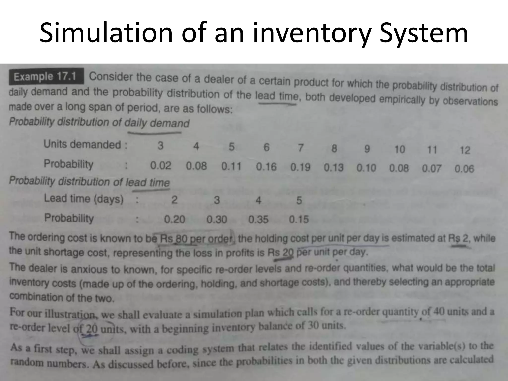
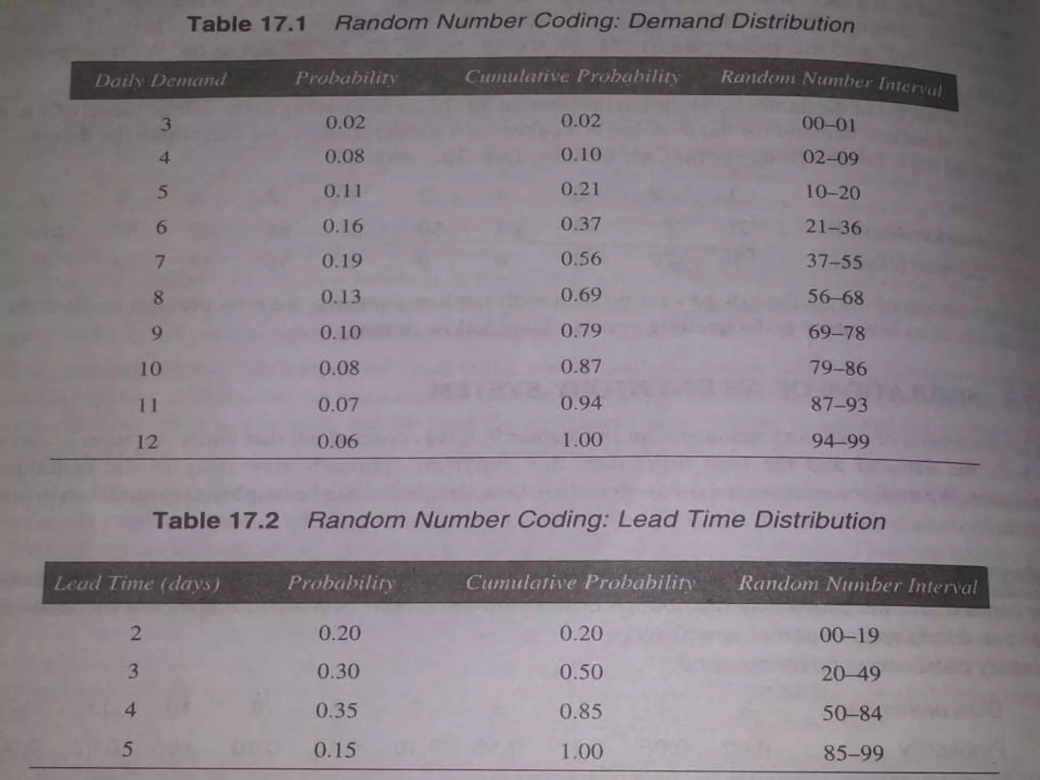
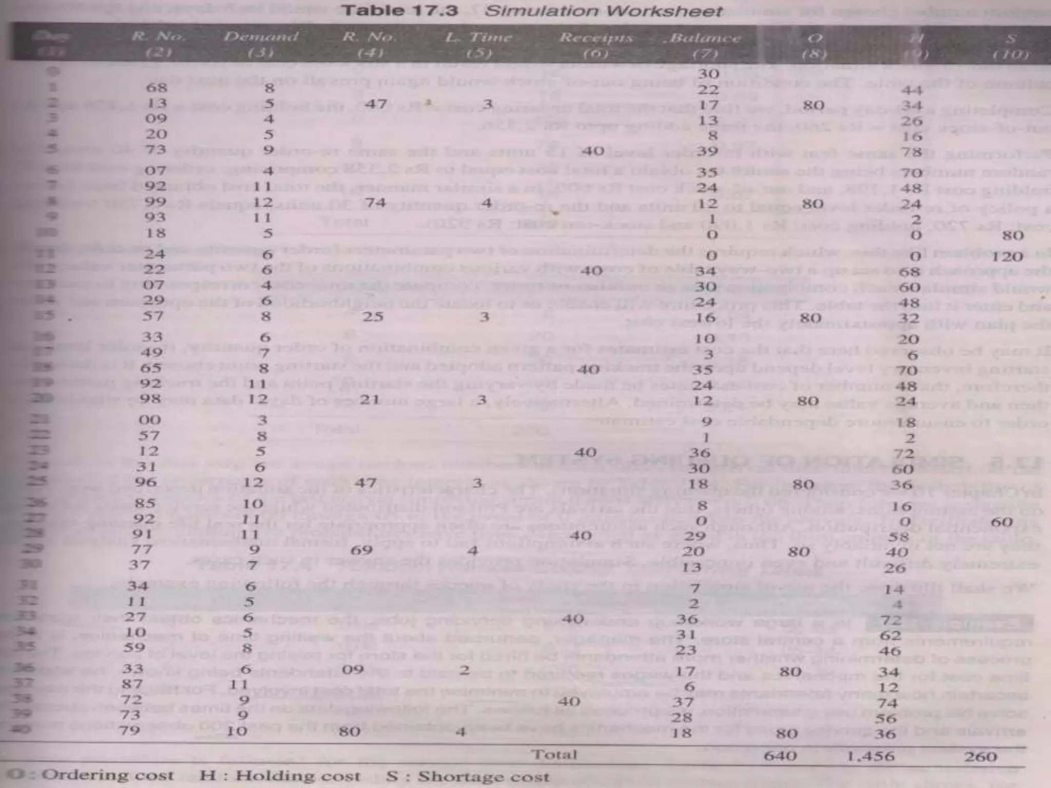
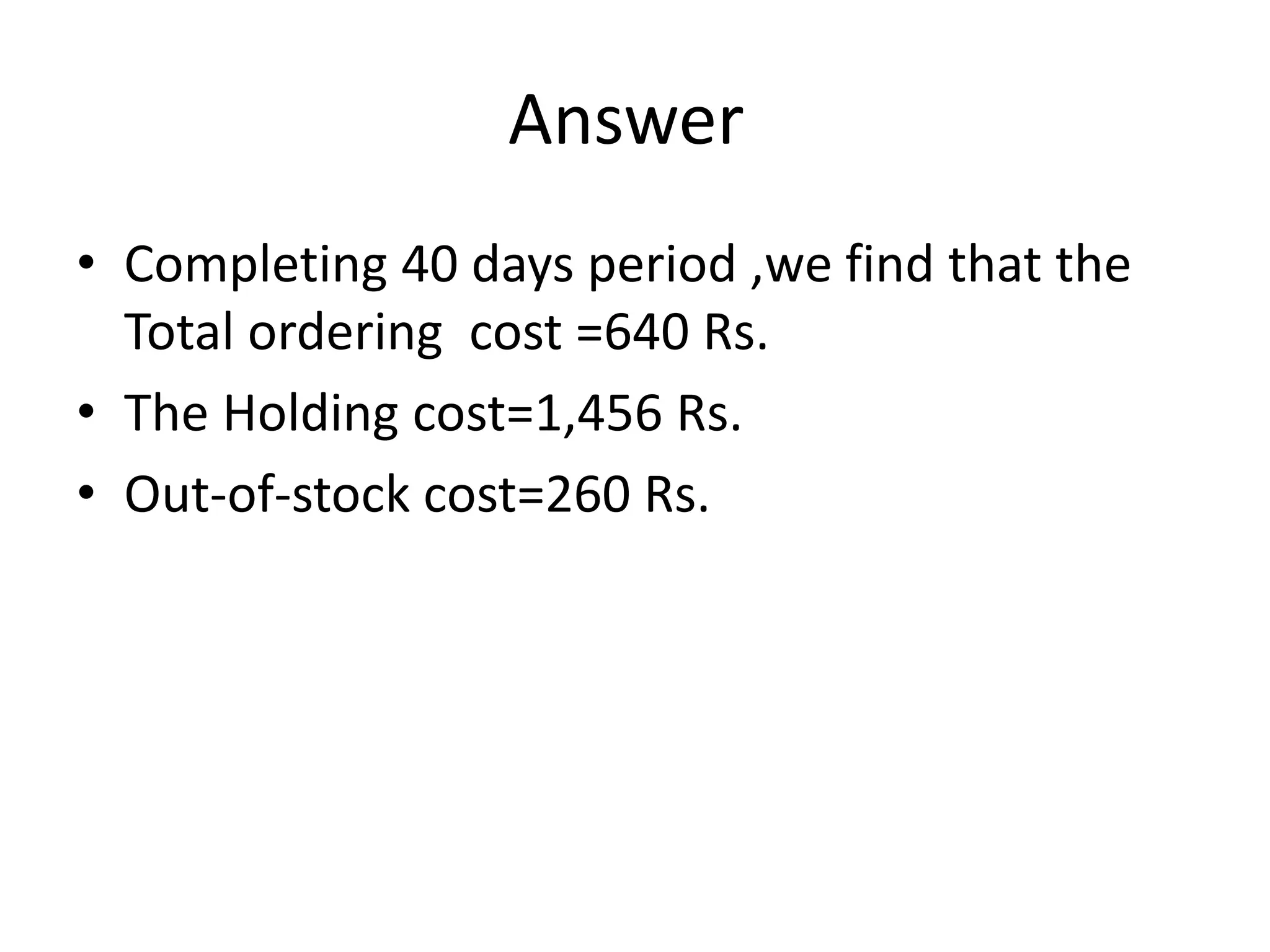
Example simulation of an inventory system with cost analyses.
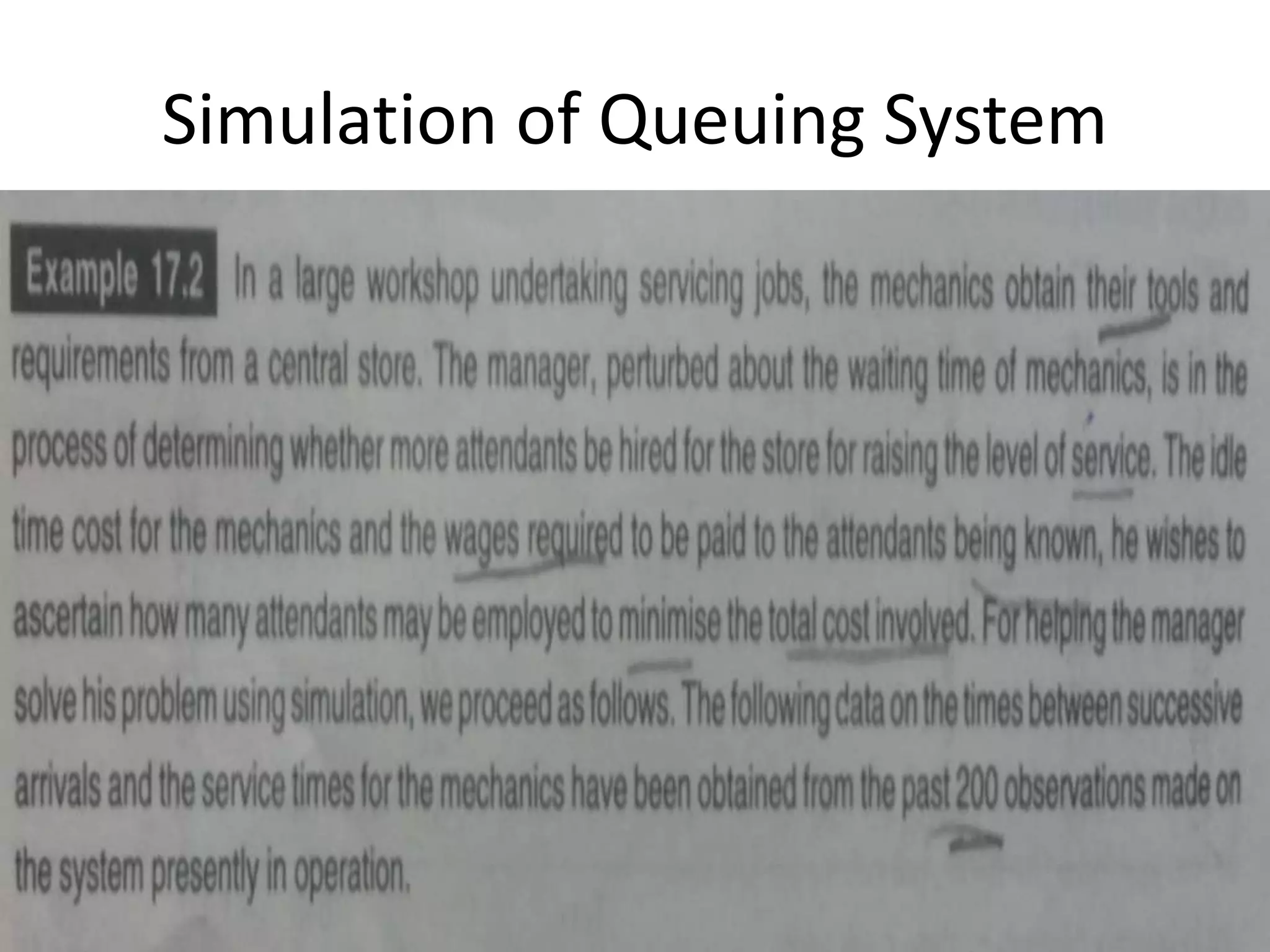
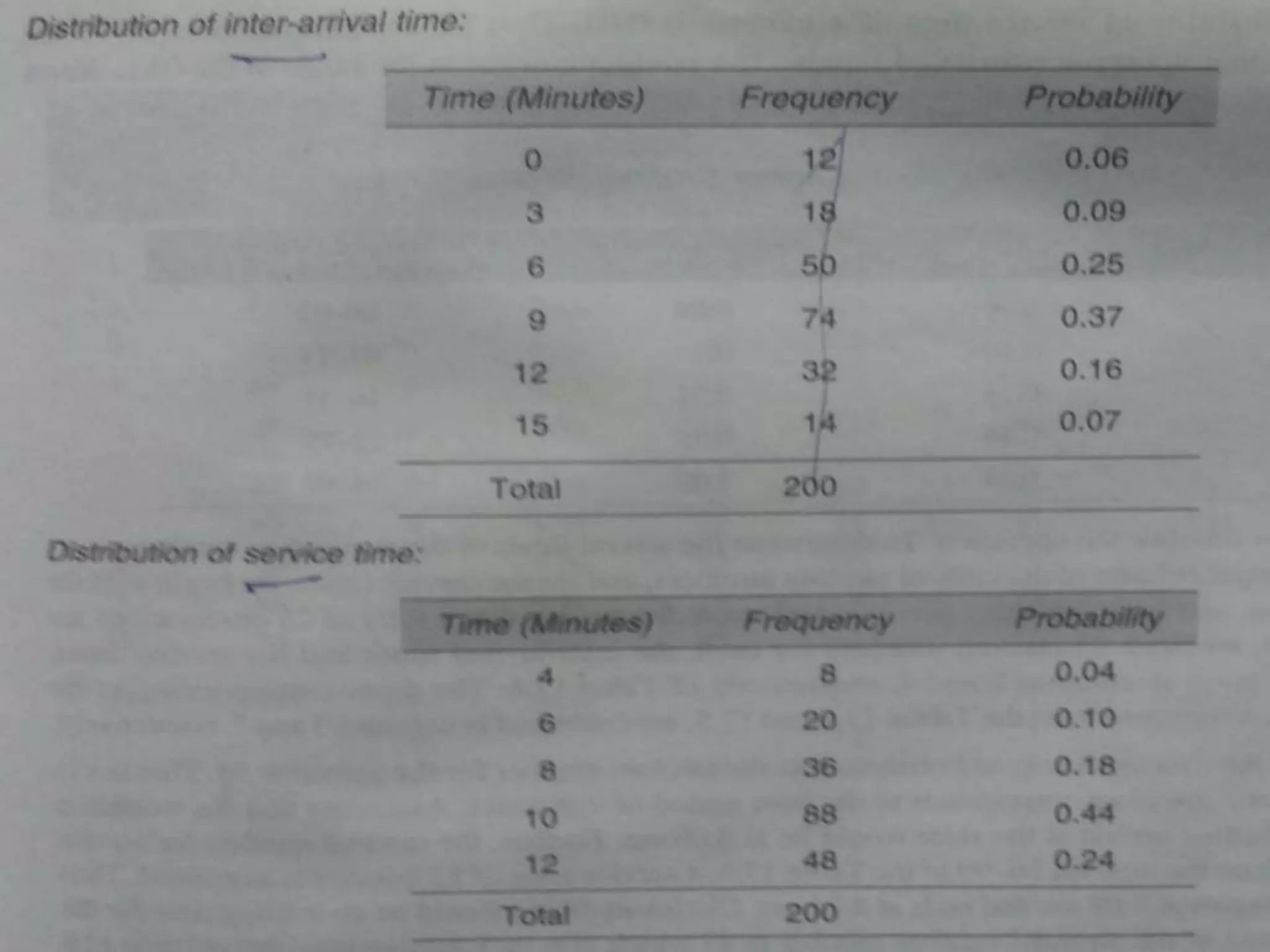
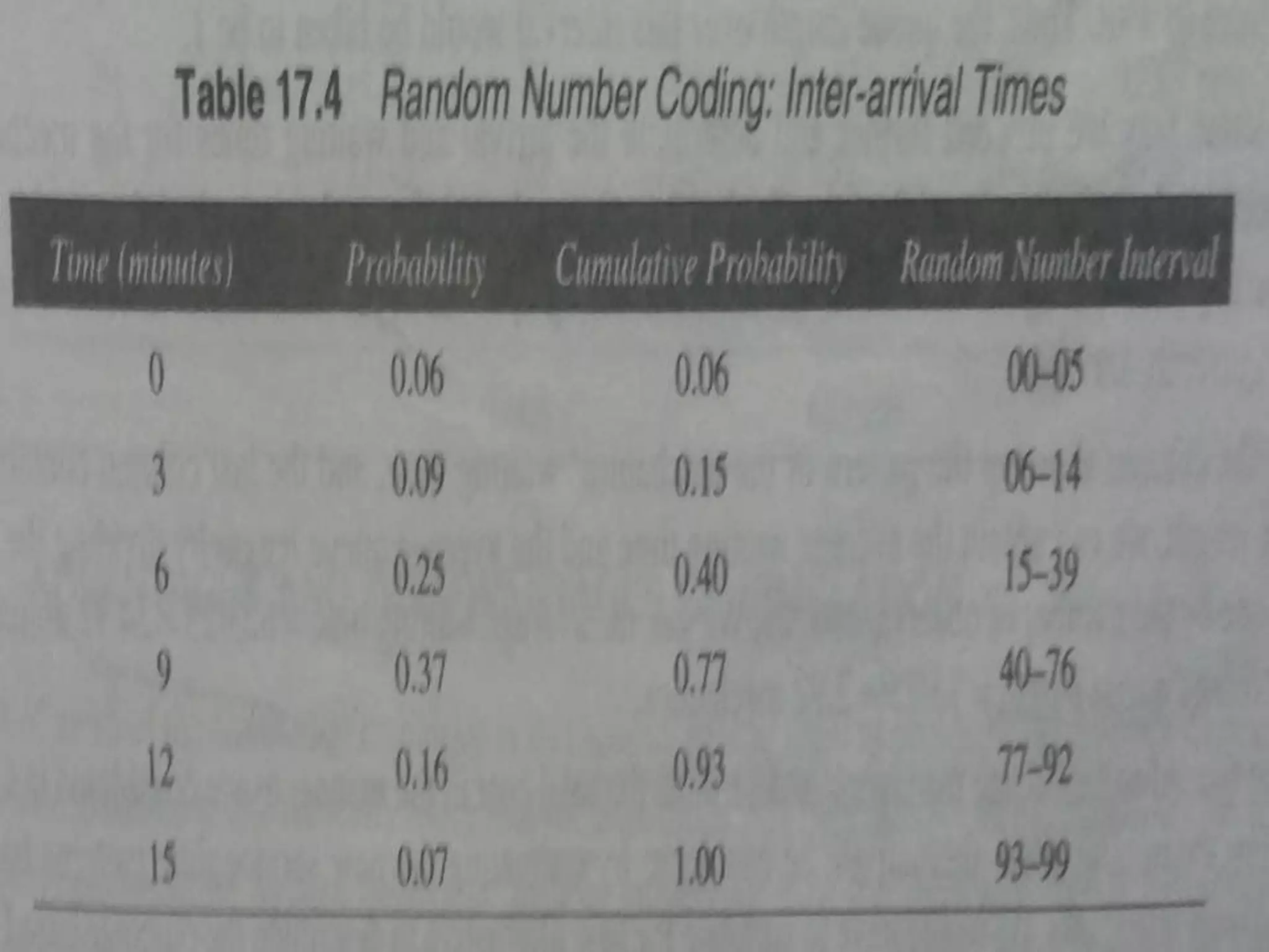
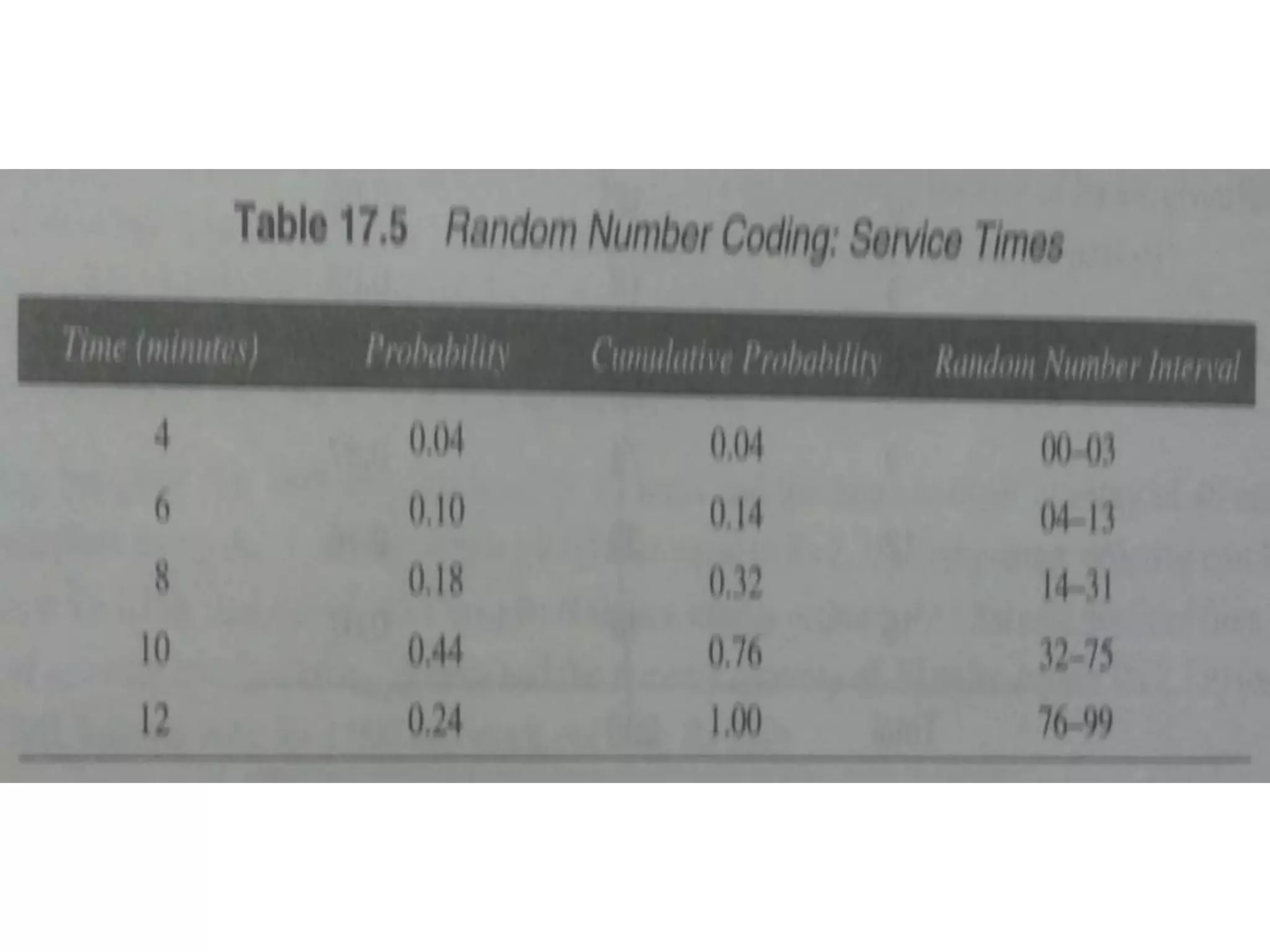
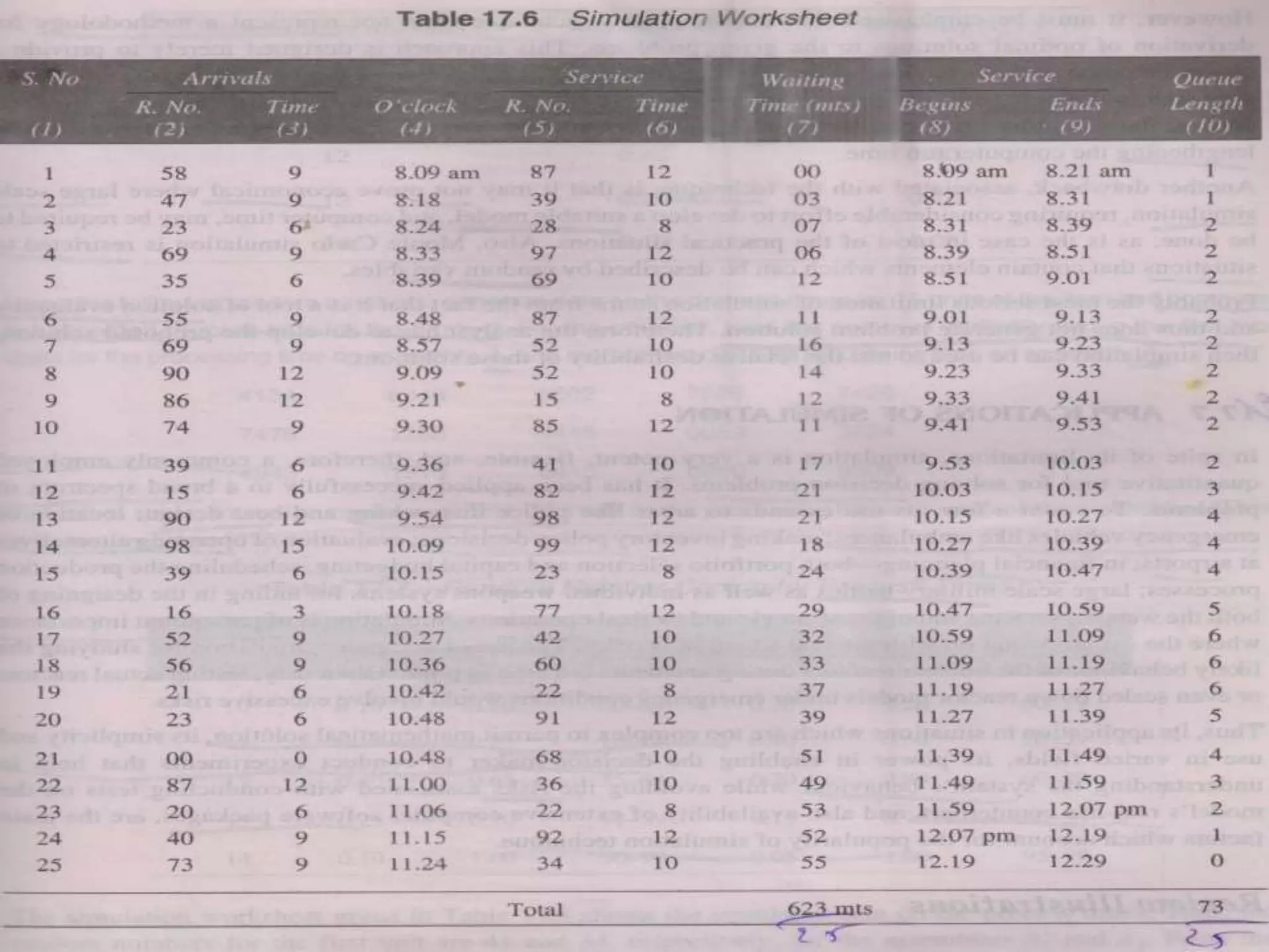
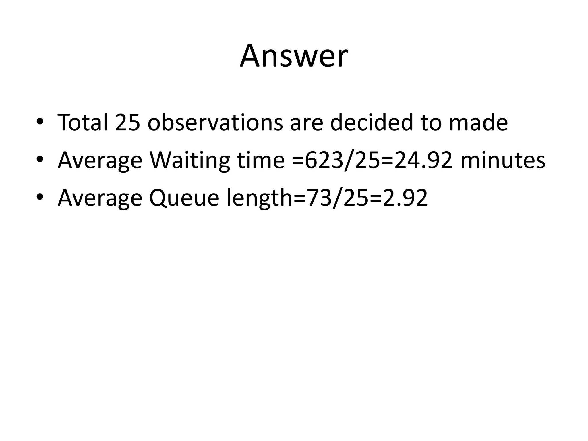
Simulation of a queuing system detailing average waiting times and queue lengths.
Queuing Theory
(Waiting LineModels)
Prepared By:
SANKET B. SUTHAR
Assistant Professor
I.T. Department,
CSPIT,CHANGA
2.
• Queuing theoryis the mathematical study of waiting
lines which are the most frequently encountered
problems in everyday life.
• For example, queue at a cafeteria, library, bank, etc.
• Common to all of these cases are the arrivals of objects
requiring service and the attendant delays when the
service mechanism is busy.
• Waiting lines cannot be eliminated completely, but
suitable techniques can be used to reduce the waiting
time of an object in the system.
• A long waiting line may result in loss of customers to
an organization. Waiting time can be reduced by
providing additional service facilities, but it may result
in an increase in the idle time of the service
mechanism.
3.
Basic Terminology: Queuingtheory (Waiting Line
Models)
• The present section focuses on the standard
vocabulary of Waiting Line Models (Queuing
Theory).
4.
Queuing Model
• Itis a suitable model used to represent a
service oriented problem, where customers
arrive randomly to receive some service, the
service time being also a random variable.
Arrival
• The statistical pattern of the arrival can be
indicated through the probability distribution
of the number of the arrivals in an interval.
5.
Service Time
- Thetime taken by a server to complete
service is known as service time.
Server
• It is a mechanism through which service is
offered.
Queue Discipline
• It is the order in which the members of the
queue are offered service.
6.
Poisson Process
• Itis a probabilistic phenomenon where the
number of arrivals in an interval of length t
follows a Poisson distribution with parameter λt,
where λ is the rate of arrival.
Queue
• A group of items waiting to receive service,
including those receiving the service, is known as
queue.
Waiting time in queue
• Time spent by a customer in the queue before
being served.
7.
Waiting time inthe system
• It is the total time spent by a customer in the
system. It can be calculated as follows:
Waiting time in the system = Waiting time in
queue + Service time
• Queue length
• Number of persons in the system at any time.
• Average length of line
• The number of customers in the queue per
unit of time.
8.
• Average idletime
• The average time for which the system
remains idle.
• FIFO
• It is the first in first out queue discipline.
• Bulk Arrivals
• If more than one customer enter the system at
an arrival event, it is known as bulk arrivals.
Please note that bulk arrivals are not
embodied in the models of the subsequent
sections.
9.
Queuing System Components
•Input Source: The input source generates
customers for the service mechanism.
• The most important characteristic of the input
source is its size. It may be either finite or infinite.
(Please note that the calculations are far easier
for the infinite case, therefore, this assumption is
often made even when the actual size is relatively
large. If the population size is finite, then the
analysis of queuing model becomes more
involved.)
• The statistical pattern by which calling units are
generated over time must also be specified. It
may be Poisson or Exponential probability
distribution.
10.
• Queue: Itis characterized by the maximum
permissible number of units that it can
contain. Queues may be infinite or finite.
• Service Discipline: It refers to the order in
which members of the queue are selected for
service. Frequently, the discipline is first come,
first served.
Following are some other disciplines:
• LIFO (Last In First Out)
• SIRO (Service In Random Order)
• Priority System
11.
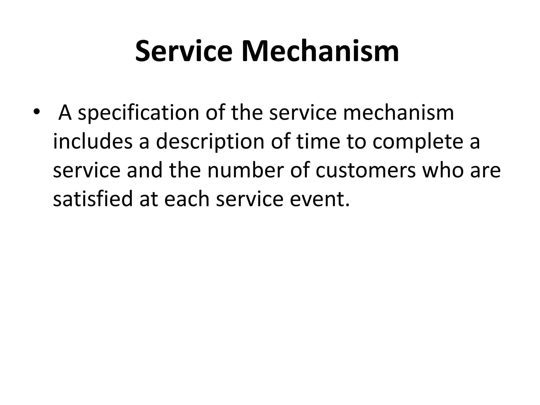
Service Mechanism
• Aspecification of the service mechanism
includes a description of time to complete a
service and the number of customers who are
satisfied at each service event.
13.
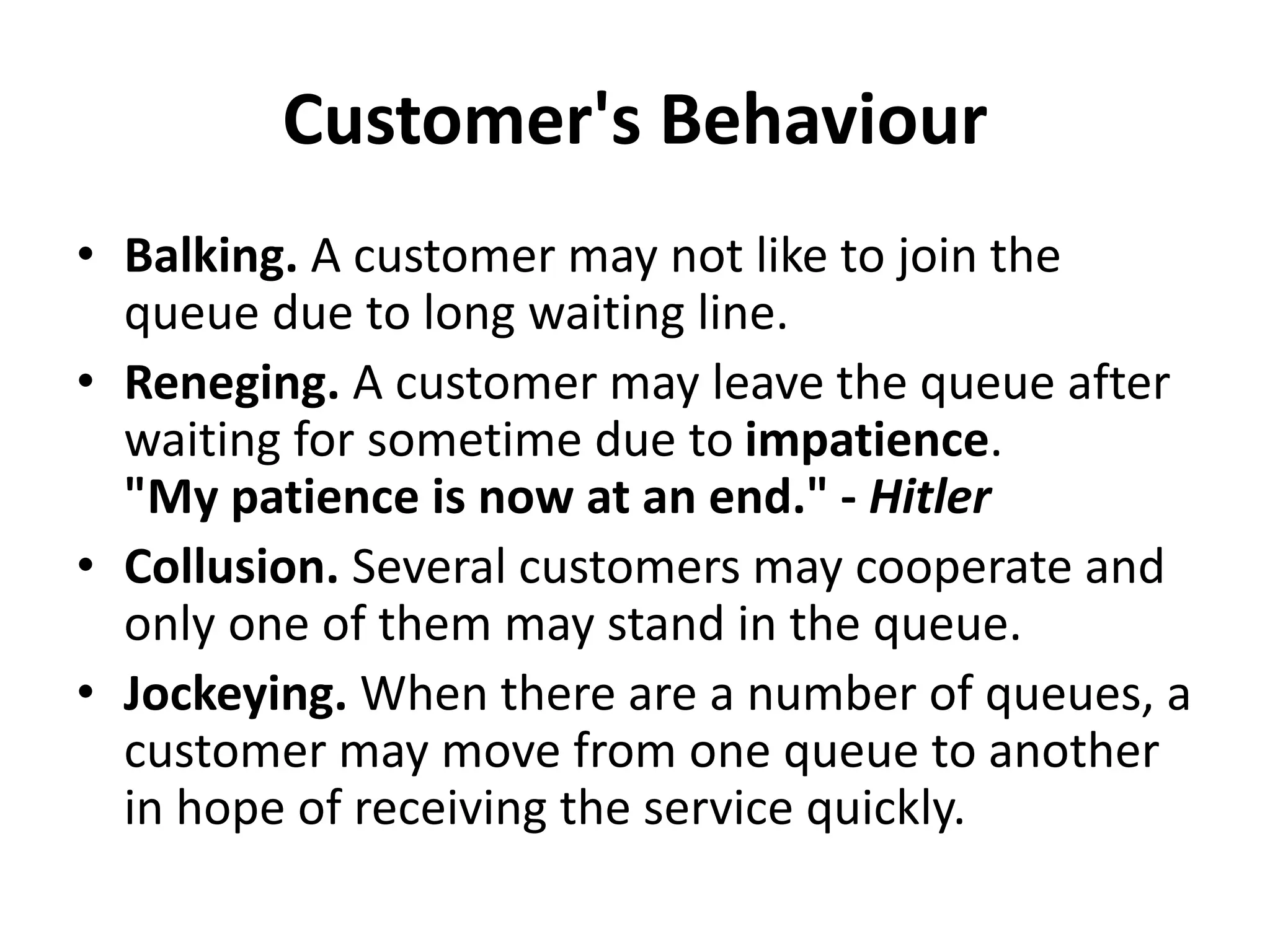
Customer's Behaviour
• Balking.A customer may not like to join the
queue due to long waiting line.
• Reneging. A customer may leave the queue after
waiting for sometime due to impatience.
"My patience is now at an end." - Hitler
• Collusion. Several customers may cooperate and
only one of them may stand in the queue.
• Jockeying. When there are a number of queues, a
customer may move from one queue to another
in hope of receiving the service quickly.
14.
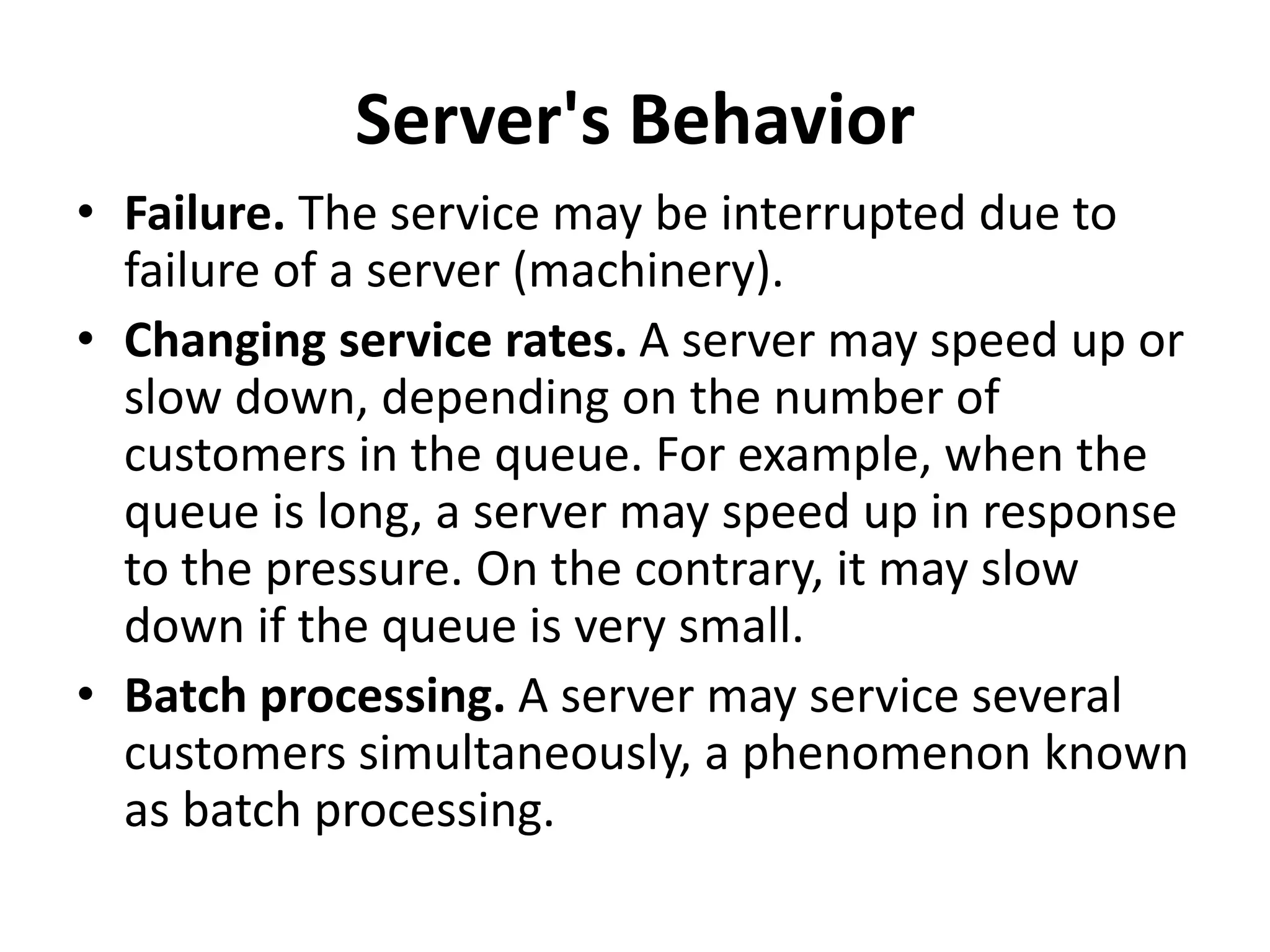
Server's Behavior
• Failure.The service may be interrupted due to
failure of a server (machinery).
• Changing service rates. A server may speed up or
slow down, depending on the number of
customers in the queue. For example, when the
queue is long, a server may speed up in response
to the pressure. On the contrary, it may slow
down if the queue is very small.
• Batch processing. A server may service several
customers simultaneously, a phenomenon known
as batch processing.
15.
Assumptions of QueuingTheory
• The source population has infinite size.
• The inter-arrival time has an exponential probability
distribution with a mean arrival rate of l customer arrivals
per unit time.
• There is no unusual customer behaviour.
• The service discipline is FIFO.
• The service time has an exponential probability distribution
with a mean service rate of m service completions per unit
time.
• The mean arrival rate is less than the mean service rate,
i.e., l < m.
• There is no unusual server behavior.
16.
Example Queuing DisciplineSpecifications
• M/D/5/40/200/FCFS
• – Exponentially distributed interval times
• – Deterministic service times
• – Five servers
• – Forty buffers (35 for waiting)
• – Total population of 200 customers
• – First-come-first-serve service discipline
• • M/M/1
• – Exponentially distributed interval times
• – Exponentially distributed service times
• – One server
• – Infinite number of buffers
• – Infinite population size
• – First-come-first-serve service discipline
17.
Notations
• N=number ofcustomers in system
• Pn=probability of n customers in the system
• λ = average (expected)customer arrival rate or
average number of arrival per unit of time in
the queuing system
• µ=average(expected)service rate or average
number of customers served per unit time at
the place of service
• λ /µ=ρ=(Average service completion
time(1/µ)) / (Average inter-arrival time(1/ λ))
18.
• S=number ofservice channels(service facilities
or servers)
• N=maximum number of customers allowed
• Ls=average (Expected)number of customers in
the system
• Lq=average (Expected)number of customers in
queue
• Lb=average (Expected)length of non-empty
queue
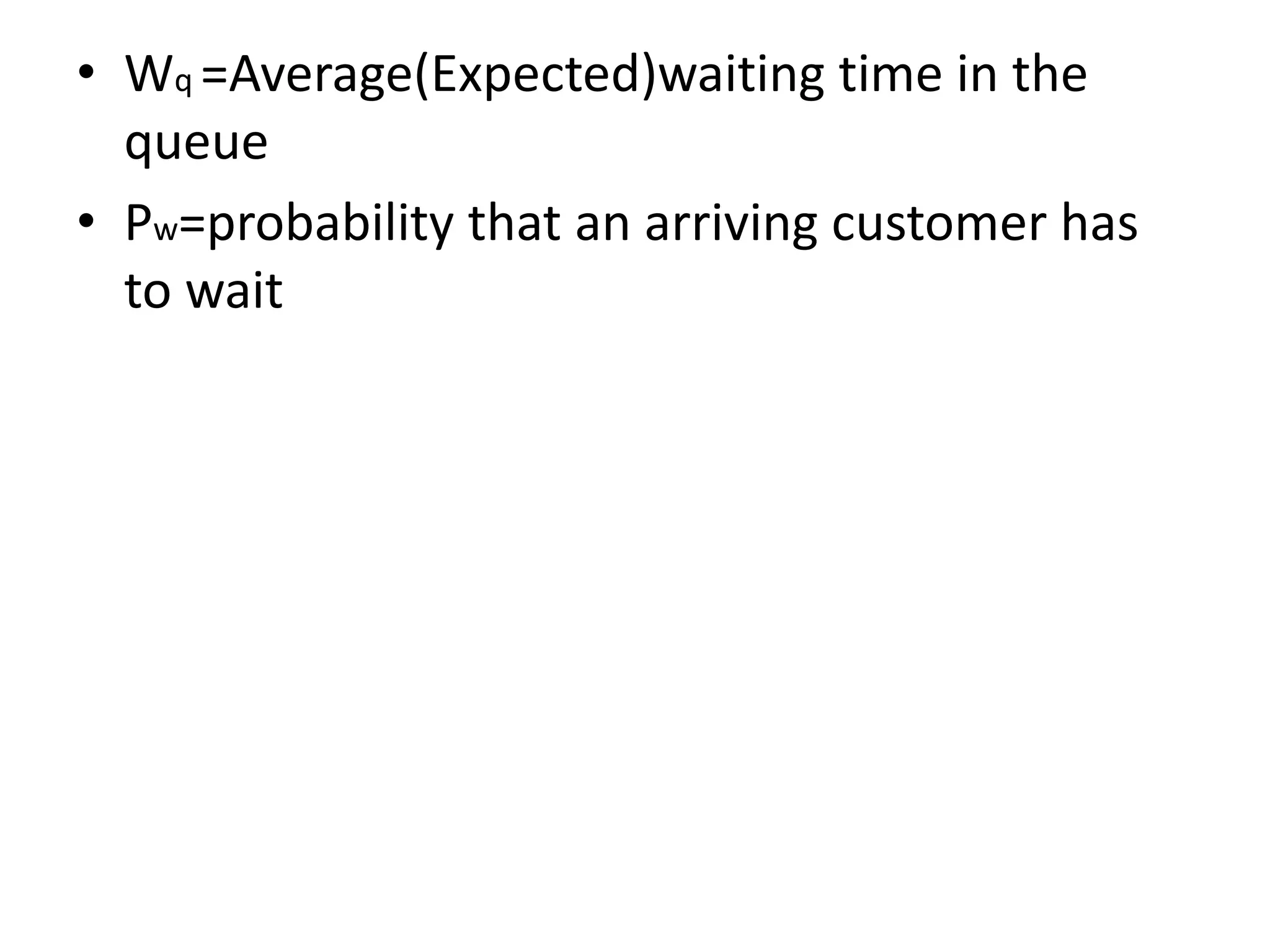
• Ws=average (Expected)waiting time in the
system
M/M/1 (∞/FIFO) QueuingSystem
• It is a queuing model where the arrivals follow a
Poisson process, service times are exponentially
distributed and there is only one server. In other
words, it is a system with Poisson input,
exponential waiting time and Poisson output with
single channel.
• Queue capacity of the system is infinite with first
in first out mode. The first M in the notation
stands for Poisson input, second M for Poisson
output, 1 for the number of servers and ∞ for
infinite capacity of the system.
21.
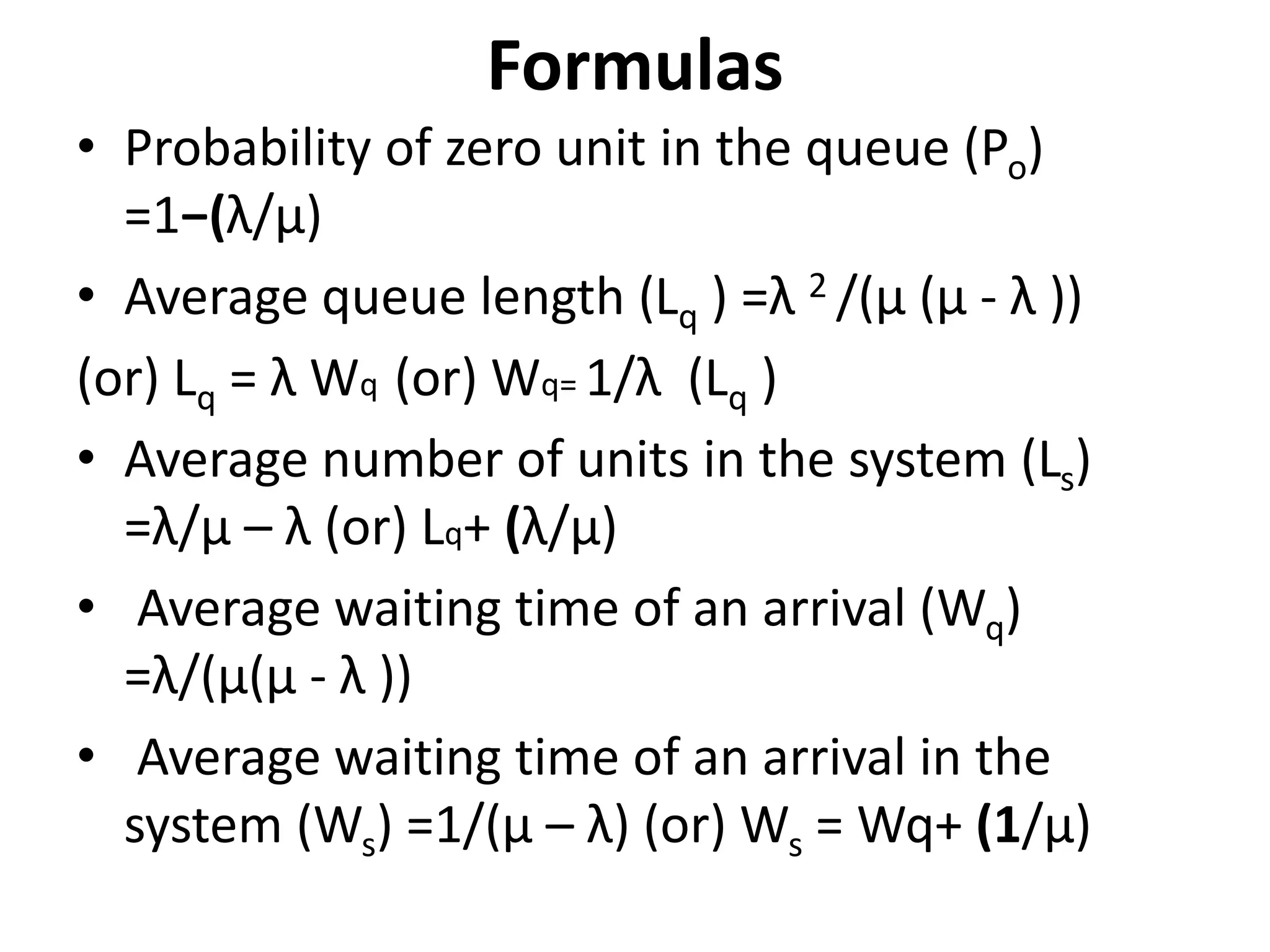
Formulas
• Probability ofzero unit in the queue (Po)
=1−(λ/μ)
• Average queue length (Lq ) =λ 2 /(μ (μ - λ ))
(or) Lq = λ Wq (or) Wq= 1/λ (Lq )
• Average number of units in the system (Ls)
=λ/μ – λ (or) Lq+ (λ/μ)
• Average waiting time of an arrival (Wq)
=λ/(μ(μ - λ ))
• Average waiting time of an arrival in the
system (Ws) =1/(μ – λ) (or) Ws = Wq+ (1/μ)
22.
Example 1
• Studentsarrive at the head office
of www.universalteacher.com according to a
Poisson input process with a mean rate of 40 per
hour. The time required to serve a student has an
exponential distribution with a mean of 50 per
hour. Assume that the students are served by a
single individual, find the average waiting time of
a student.
Solution:
Given
λ = 40/hour, μ = 50/hour
Average waiting time of a student before receiving
service (Wq) =40/(50(50 - 40))=4.8 minutes
23.
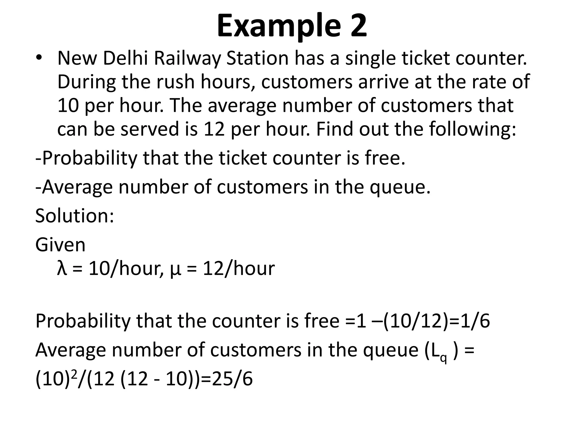
Example 2
• NewDelhi Railway Station has a single ticket counter.
During the rush hours, customers arrive at the rate of
10 per hour. The average number of customers that
can be served is 12 per hour. Find out the following:
-Probability that the ticket counter is free.
-Average number of customers in the queue.
Solution:
Given
λ = 10/hour, μ = 12/hour
Probability that the counter is free =1 –(10/12)=1/6
Average number of customers in the queue (Lq ) =
(10)2/(12 (12 - 10))=25/6
24.
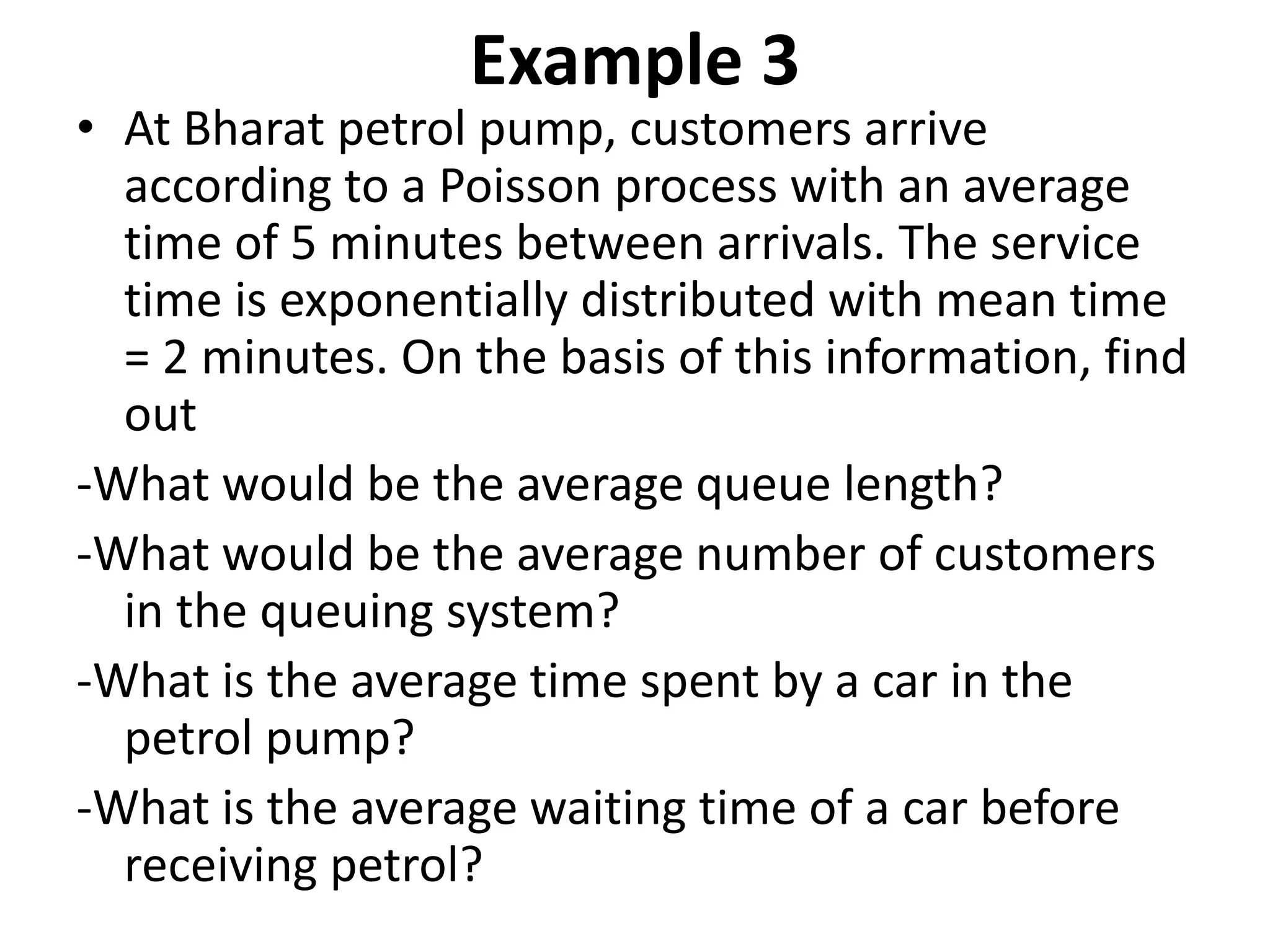
Example 3
• AtBharat petrol pump, customers arrive
according to a Poisson process with an average
time of 5 minutes between arrivals. The service
time is exponentially distributed with mean time
= 2 minutes. On the basis of this information, find
out
-What would be the average queue length?
-What would be the average number of customers
in the queuing system?
-What is the average time spent by a car in the
petrol pump?
-What is the average waiting time of a car before
receiving petrol?
25.
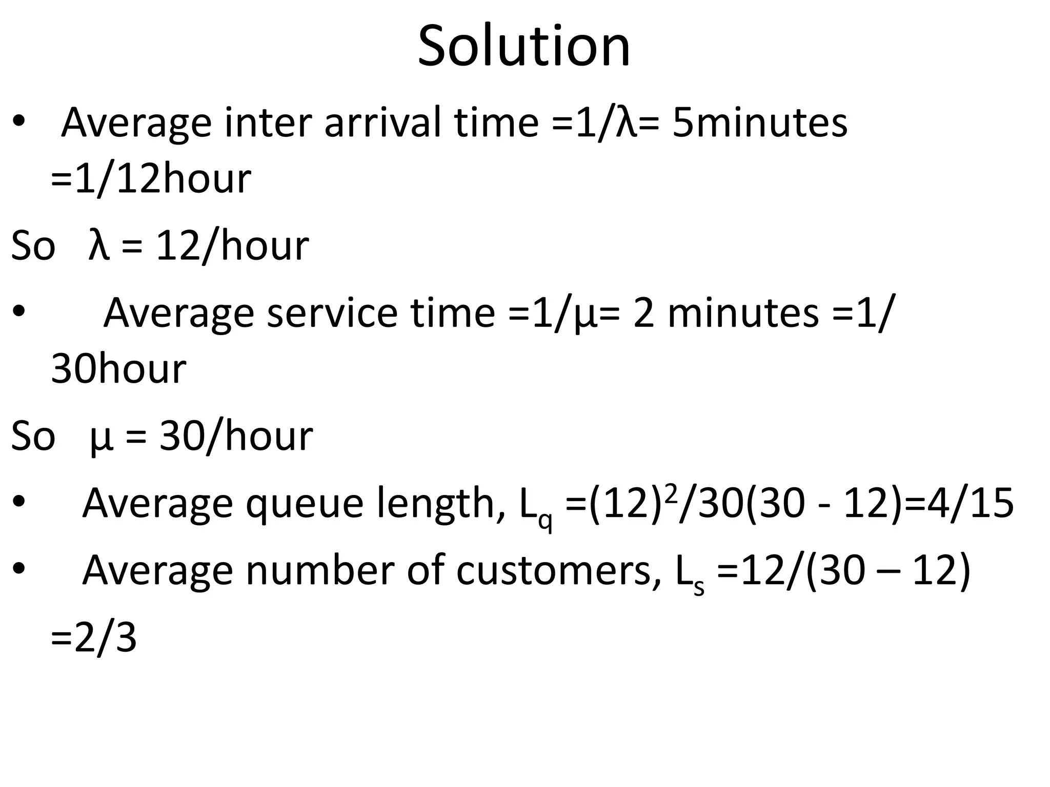
Solution
• Average interarrival time =1/λ= 5minutes
=1/12hour
So λ = 12/hour
• Average service time =1/μ= 2 minutes =1/
30hour
So μ = 30/hour
• Average queue length, Lq =(12)2/30(30 - 12)=4/15
• Average number of customers, Ls =12/(30 – 12)
=2/3
26.
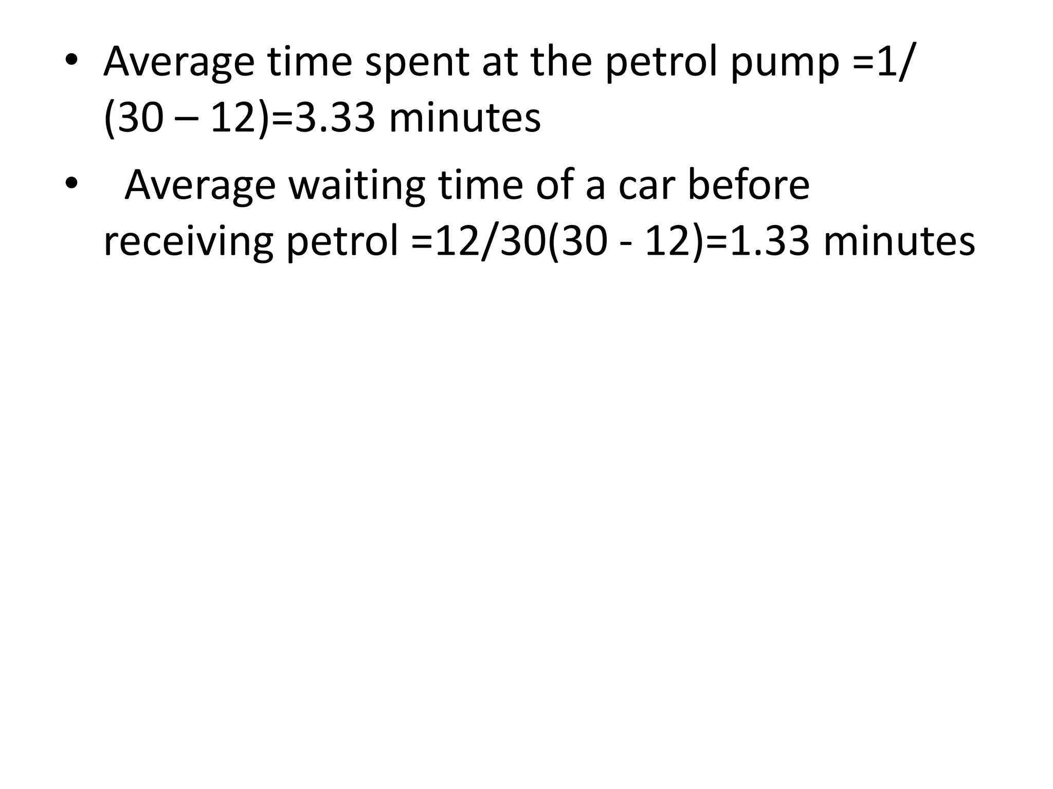
• Average timespent at the petrol pump =1/
(30 – 12)=3.33 minutes
• Average waiting time of a car before
receiving petrol =12/30(30 - 12)=1.33 minutes
27.
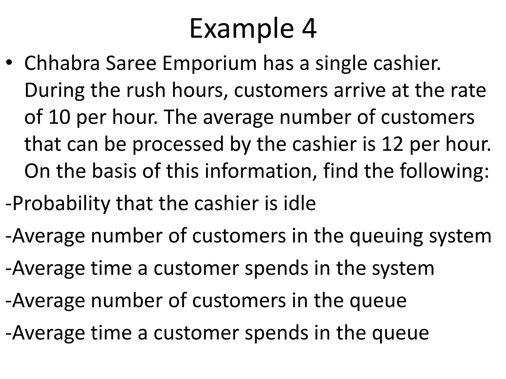
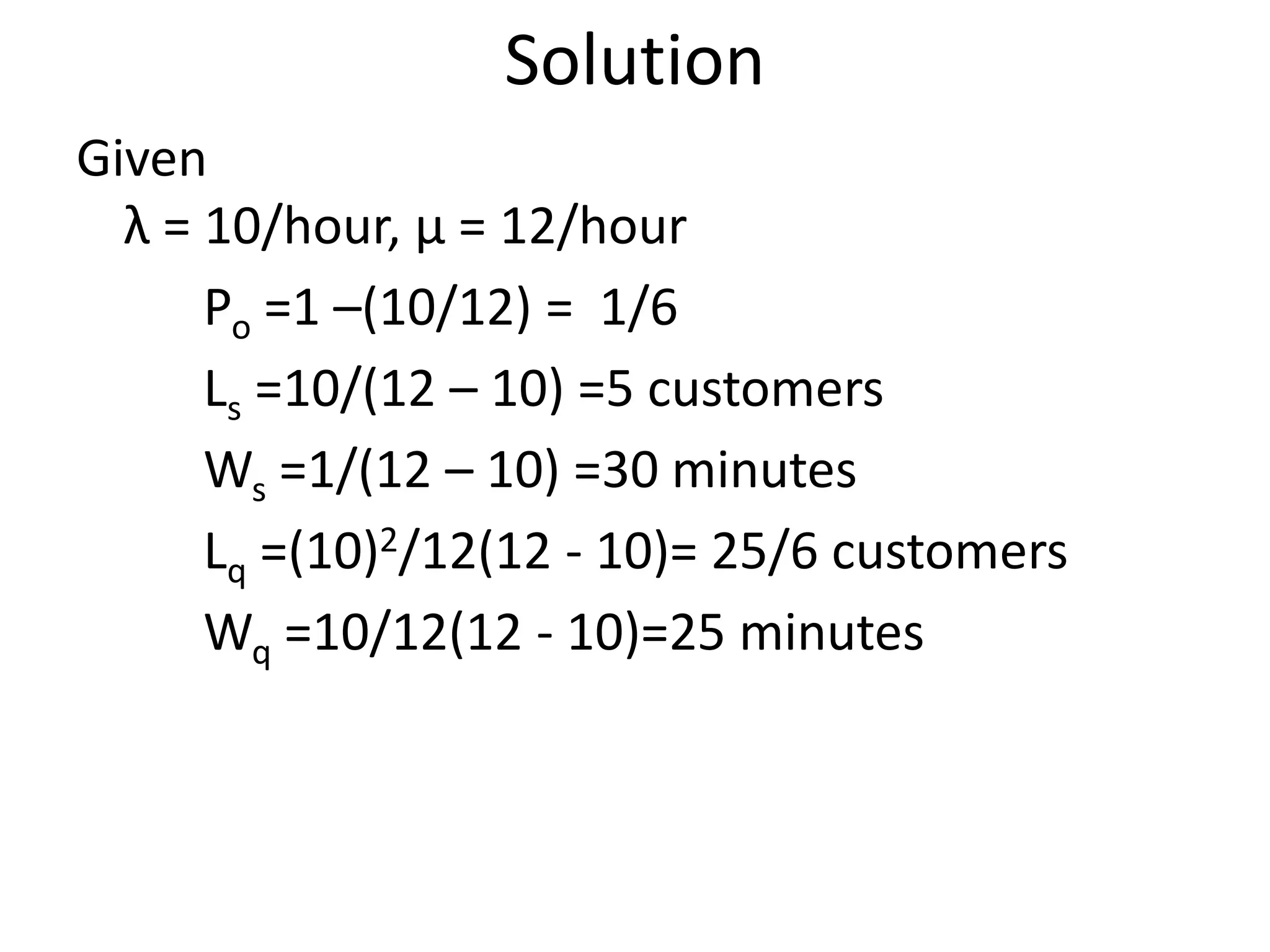
Example 4
• ChhabraSaree Emporium has a single cashier.
During the rush hours, customers arrive at the rate
of 10 per hour. The average number of customers
that can be processed by the cashier is 12 per hour.
On the basis of this information, find the following:
-Probability that the cashier is idle
-Average number of customers in the queuing system
-Average time a customer spends in the system
-Average number of customers in the queue
-Average time a customer spends in the queue
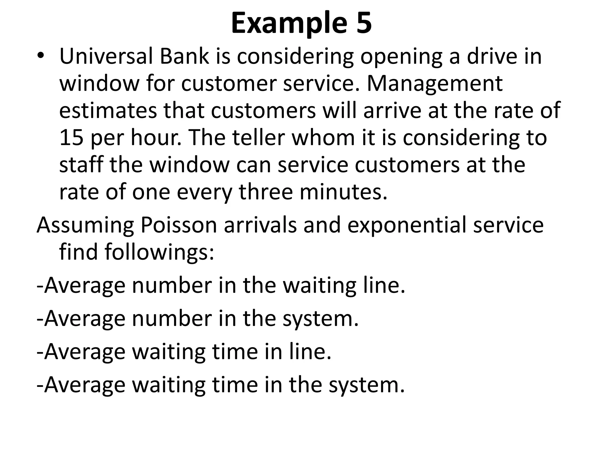
Example 5
• UniversalBank is considering opening a drive in
window for customer service. Management
estimates that customers will arrive at the rate of
15 per hour. The teller whom it is considering to
staff the window can service customers at the
rate of one every three minutes.
Assuming Poisson arrivals and exponential service
find followings:
-Average number in the waiting line.
-Average number in the system.
-Average waiting time in line.
-Average waiting time in the system.
30.
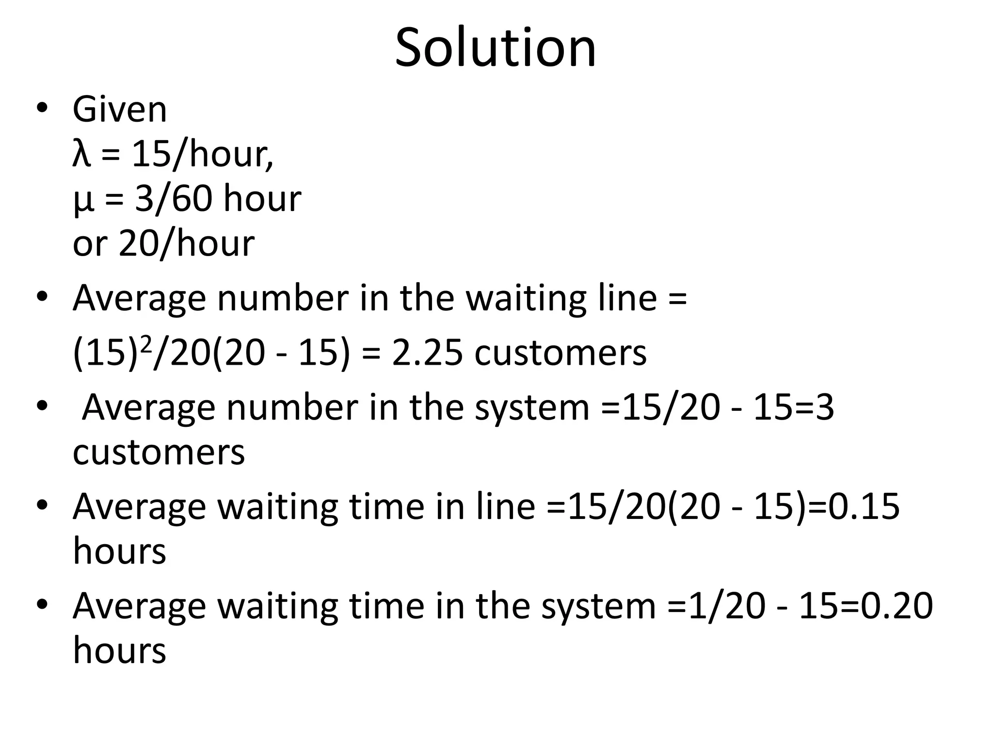
Solution
• Given
λ =15/hour,
μ = 3/60 hour
or 20/hour
• Average number in the waiting line =
(15)2/20(20 - 15) = 2.25 customers
• Average number in the system =15/20 - 15=3
customers
• Average waiting time in line =15/20(20 - 15)=0.15
hours
• Average waiting time in the system =1/20 - 15=0.20
hours
31.
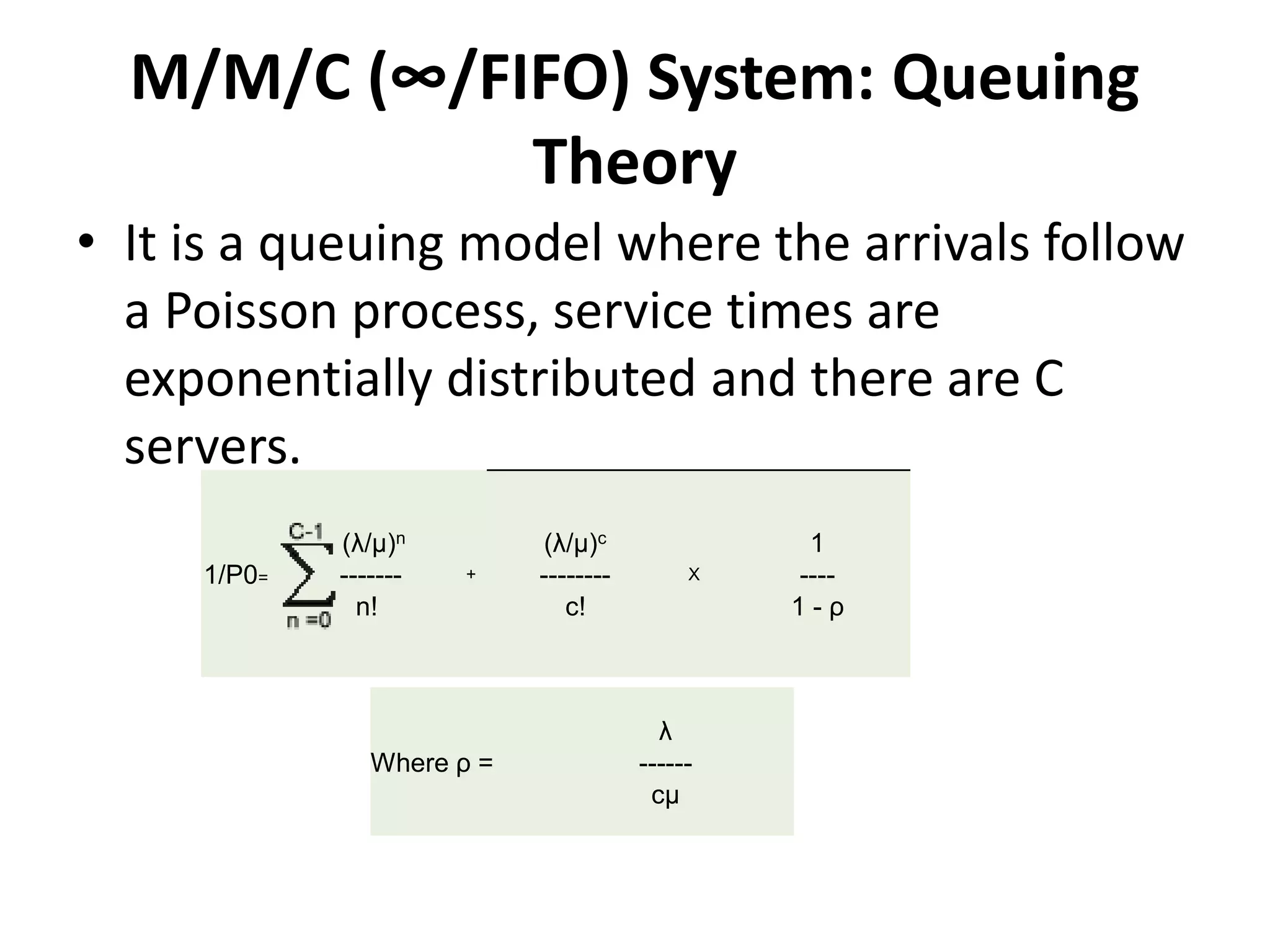
M/M/C (∞/FIFO) System:Queuing
Theory
• It is a queuing model where the arrivals follow
a Poisson process, service times are
exponentially distributed and there are C
servers.
1/P0=
(λ/μ)n
- -------
n!
+
(λ/μ)c
--------
c!
X
1
----
1 - ρ
Where ρ =
λ
------
cμ
32.
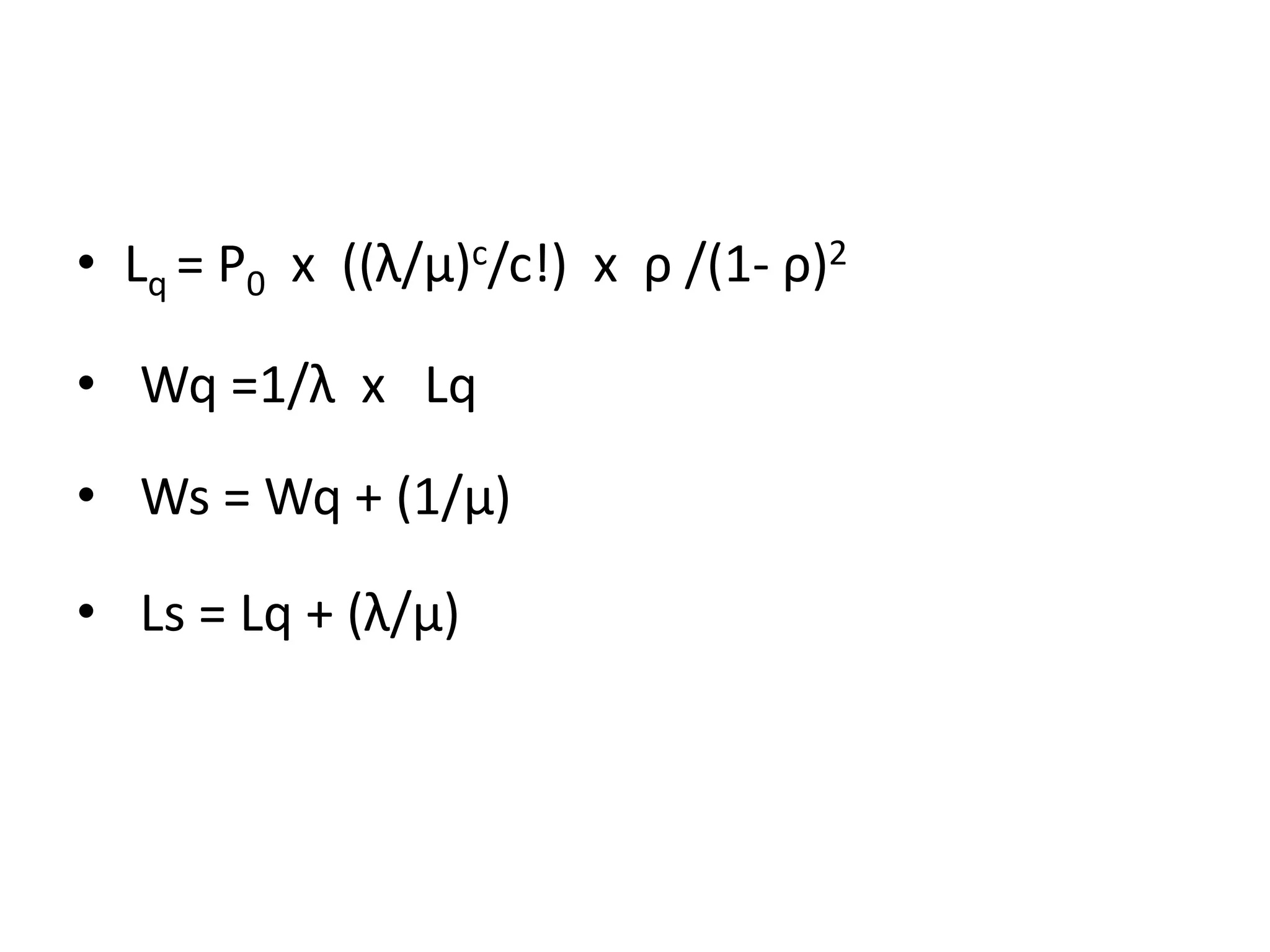
• Lq =P0 x ((λ/μ)c/c!) x ρ /(1- ρ)2
• Wq =1/λ x Lq
• Ws = Wq + (1/μ)
• Ls = Lq + (λ/μ)
33.
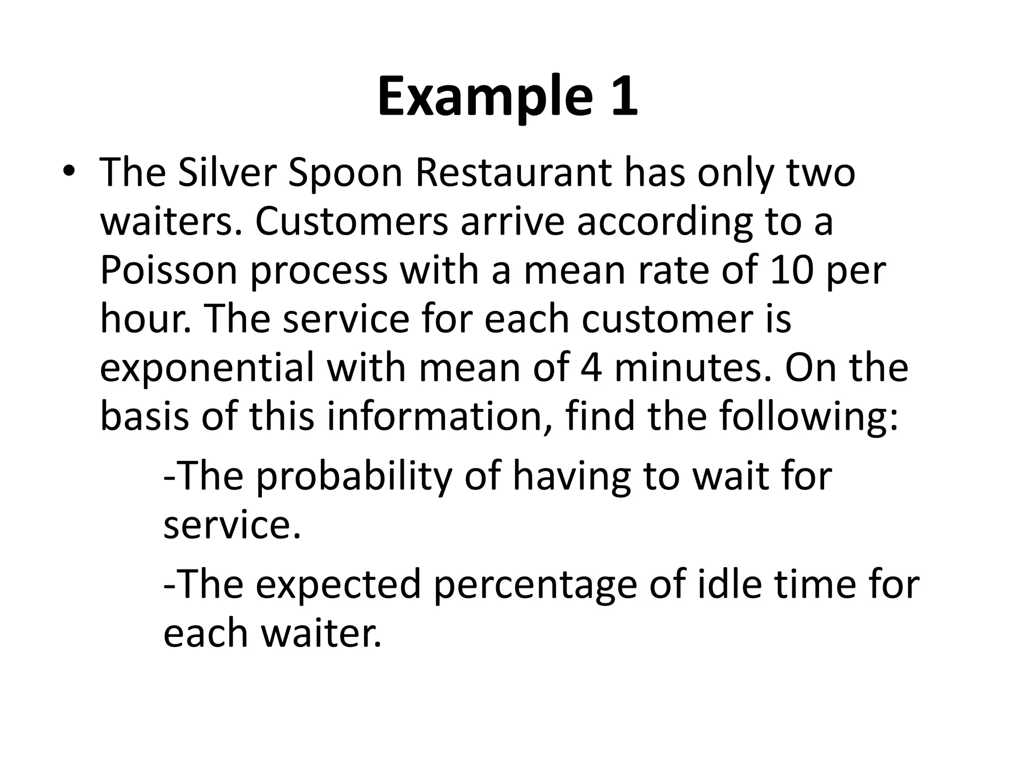
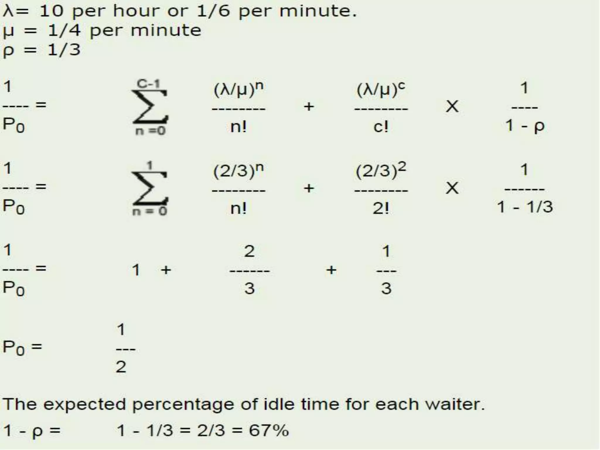
Example 1
• TheSilver Spoon Restaurant has only two
waiters. Customers arrive according to a
Poisson process with a mean rate of 10 per
hour. The service for each customer is
exponential with mean of 4 minutes. On the
basis of this information, find the following:
-The probability of having to wait for
service.
-The expected percentage of idle time for
each waiter.
35.
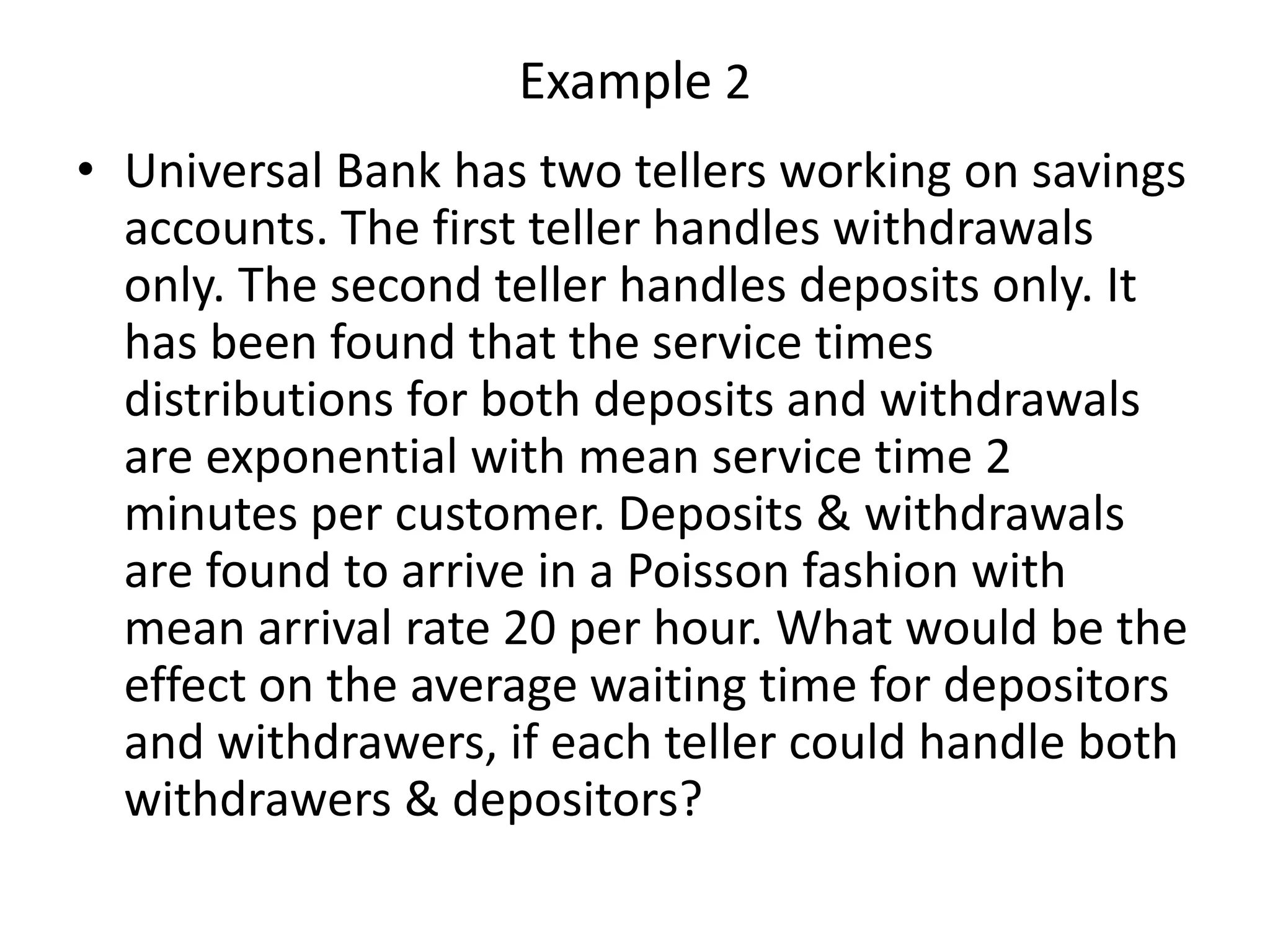
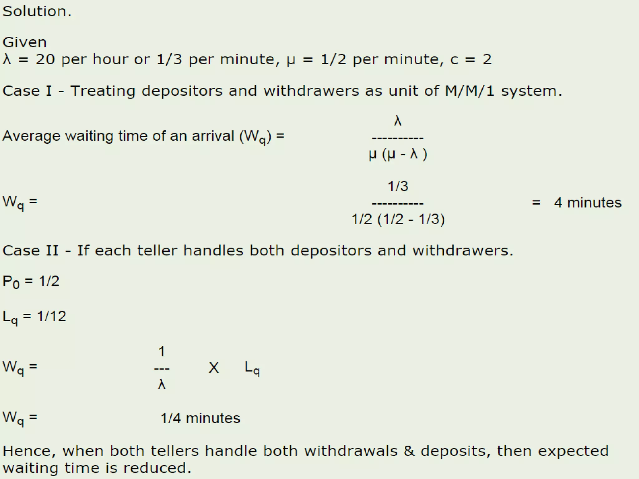
Example 2
• UniversalBank has two tellers working on savings
accounts. The first teller handles withdrawals
only. The second teller handles deposits only. It
has been found that the service times
distributions for both deposits and withdrawals
are exponential with mean service time 2
minutes per customer. Deposits & withdrawals
are found to arrive in a Poisson fashion with
mean arrival rate 20 per hour. What would be the
effect on the average waiting time for depositors
and withdrawers, if each teller could handle both
withdrawers & depositors?
Outline for Today’sTalk
• Definition of Simulation
• Brief History
• Applications
• “Real World” Applications
• Example of how to build one
• Questions????
39.
Definition:
“Simulation is theprocess of designing
a model of a real system and conducting
experiments with this model for the
purpose of either understanding the
behavior of the system and/or
evaluating various strategies for the
operation of the system.”
- Introduction to Simulation Using SIMAN
(2nd Edition)
40.
Allows us to:
•Model complex systems in a detailed way
• Describe the behavior of systems
• Construct theories or hypotheses that account for
the observed behavior
• Use the model to predict future behavior, that is,
the effects that will be produced by changes in
the system
• Analyze proposed systems
41.
Simulation is oneof the most widely
used techniques in operations research
and management science…
42.
Brief History Nota very old technique...
• World War II
• “Monte Carlo” simulation: originated with
the work on the atomic bomb. Used to
simulate bombing raids. Given the
security code name “Monte-Carlo”.
• Still widely used today for certain problems
which are not analytically solvable (for
example: complex multiple integrals…)
43.
Brief History (cont.)
•Late ‘50s, early ‘60s
• Computers improve
• First languages introduced: SIMSCRIPT, GPSS (IBM)
• Simulation viewed at the tool of “last resort”
• Late ‘60s, early ‘70s
• Primary computers were mainframes: accessibility
and interaction was limited
• GASP IV introduced by Pritsker. Triggered a wave
of diverse applications. Significant in the evolution
of simulation.
44.
Brief History (cont.)
•Late ‘70s, early ‘80s
• SLAM introduced in 1979 by Pritsker and Pegden.
• Models more credible because of sophisticated tools.
• SIMAN introduced in 1982 by Pegden. First language
to run on both a mainframe as well as a
microcomputer.
• Late ‘80s through present
• Powerful PCs
• Languages are very sophisticated (market almost
saturated)
• Major advancement: graphics. Models can now be
animated!
45.
What can besimulated?
Almost anything can
and
almost everything has...
46.
Applications:
• COMPUTER SYSTEMS:hardware components, software
systems, networks, data base management, information
processing, etc..
• MANUFACTURING: material handling systems, assembly
lines, automated production facilities, inventory control
systems, plant layout, etc..
• BUSINESS: stock and commodity analysis, pricing policies,
marketing strategies, cash flow analysis, forecasting, etc..
• GOVERNMENT: military weapons and their use, military
tactics, population forecasting, land use, health care
delivery, fire protection, criminal justice, traffic control,
etc..
And the list goes on and on...
47.
Examples of Applicationsat Disney World
• Cruise Line Operation: Simulate the arrival and
check-in process at the dock. Discovered the
process they had in mind would cause hours
in delays before getting on the ship.
• Private Island Arrival: How to transport passengers
to the beach area? Drop-off point far from the
beach. Used simulation to determine whether
to invest in trams, how many trams to purchase,
average transport and waiting times, etc..
48.
Examples of Applicationsat Disney World
• Bus Maintenance Facility: Investigated “best” way
of scheduling preventative maintenance trips.
• Alien Encounter Attraction: Visitors move through
three areas. Encountered major variability
when ride opened due to load and unload
times (therefore, visitors waiting long periods
before getting on the ride). Used simulation
to determine the length of the individual shows
so as to avoid bottlenecks.
Advantages to Simulation:
•Can be used to study existing systems without disrupting the
ongoing operations.
• Proposed systems can be “tested” before committing resources.
• Allows us to control time.
• Allows us to identify bottlenecks.
• Allows us to gain insight into which variables are most
important to system performance.
Disadvantages to Simulation
•Model building is an art as well as a science. The quality
of the analysis depends on the quality of the model and the
skill of the modeler (Remember: GIGO)
• Simulation results are sometimes hard to interpret.
• Simulation analysis can be time consuming and expensive.
Should not be used when an analytical method would
provide for quicker results.
53.
Process of Simulation
Totalfour Phase of the Simulation Process
A)Definition of the problem and statement of objectives
B)Construction of an appropriate model
C)Experimentation with the model constructed
D)Evaluation of the result of Simulation