Queuing theory is the mathematical study of waiting lines in systems like customer service lines. It enables the analysis of processes like customer arrivals, waiting times, and service times. The document discusses the M/M/c queuing model, which assumes arrivals and service times follow exponential distributions and there are c parallel servers. It provides the steady state probabilities and performance measures like expected number of customers in the system and in the queue for the M/M/c model. An example applies the M/M/1 model to analyze whether a hospital should hire a second doctor based on arrival and service rates.

1. QUEUING THEORY
[M/M/C MODEL]
Student Adviser:-Assist.Prof. Sanjay Kumar
Student:-Ram Niwas Meena
Semester:-Fourth
“Delay is the enemy of efficiency” and “Waiting is the enemy of utilization”

2. 1
OVERVIEW
 What is queuing theory?
 Examples of Real World Queuing Systems?
 Components of a Basic Queuing Process
 A Commonly Seen Queuing Model
 Terminology and Notation
 Little’s Formula
 The M/M/1 – model
 Example
 M/M/c Model

3. 2
 Mathematical analysis of queues and waiting times in stochastic
systems.
 Used extensively to analyze production and service processes
exhibiting random variability in market demand (arrival times) and
service times.
 Queues arise when the short term demand for service exceeds the
capacity
 Most often caused by random variation in service times and the
times between customer arrivals.
 If long term demand for service > capacity the queue will explode!
Queuing theory is the mathematical study of waiting lines (or
queues) that enables mathematical analysis of several related
processes, including arriving at the (back of the) queue, waiting in
the queue, and being served by the Service Channels at the front
of the queue.
WHAT IS QUEUING THEORY?

4. What is Transient & Steady State of the system?
Queuing analysis involves the system’s behavior over time. If the operating
characteristics vary with time then it is said to be transient state of the system.
If the behavior becomes independent of its initial conditions (no. of customers in
the system) and of the elapsed time is called Steady State condition of the
system
What do you mean by Balking, Reneging, Jockeying?
Balking
If a customer decides not to enter the queue since it is too long is called Balking
Reneging
If a customer enters the queue but after sometimes loses patience and leaves it is
called Reneging
Jockeying
When there are 2 or more parallel queues and the customers move from one
queue to another is called Jockeying
3

5. QUEUING MODELS CALCULATE:
 Average number of customers in the system waiting and being served
 Average number of customers waiting in the line
 Average time a customer spends in the system waiting and being served
 Average time a customer spends waiting in the waiting line or queue.
 Probability no customers in the system
 Probability n customers in the system
 Utilization rate: The proportion of time the system is in use.
4

6. 5
 Commercial Queuing Systems
 Commercial organizations serving external customers
 Ex. , bank, ATM, gas stations…
 Transportation service systems
 Vehicles are customers or servers
 Ex. Vehicles waiting at toll stations and traffic lights, trucks or
ships waiting to be loaded, taxi cabs, fire engines, elevators,
buses …
 Business-internal service systems
 Customers receiving service are internal to the organization
providing the service
 Ex. Inspection stations, conveyor belts, computer support …
 Social service systems
 Ex. Judicial process, hospital, waiting lists for organ transplants
or student dorm rooms …
Examples of Real World Queuing Systems?

7. Prabhakar
Car Wash
enter exit
Population of
dirty cars
Arrivals
from the
general
population …
Queue
(waiting line)
Service
facility Exit the system
Exit the system
Arrivals to the system In the system
Arrival Characteristics
•Size of the population
•Behavior of arrivals
•Statistical distribution
of arrivals
Waiting Line
Characteristics
•Limited vs. unlimited
•Queue discipline
Service Characteristics
•Service design
•Statistical distribution of
service

8. 7
 The calling population
 The population from which customers/jobs originate
 The size can be finite or infinite (the latter is most
common)
 Can be homogeneous (only one type of customers/
jobs) or heterogeneous (several different kinds of
customers/jobs)
 The Arrival Process
 Determines how, when and where customer/jobs
arrive to the system
 Important characteristic is the customers’/jobs’ inter-
arrival times
 To correctly specify the arrival process requires data
collection of inter arrival times and statistical analysis.
Components of a Basic Queuing Process (II)

9. 8
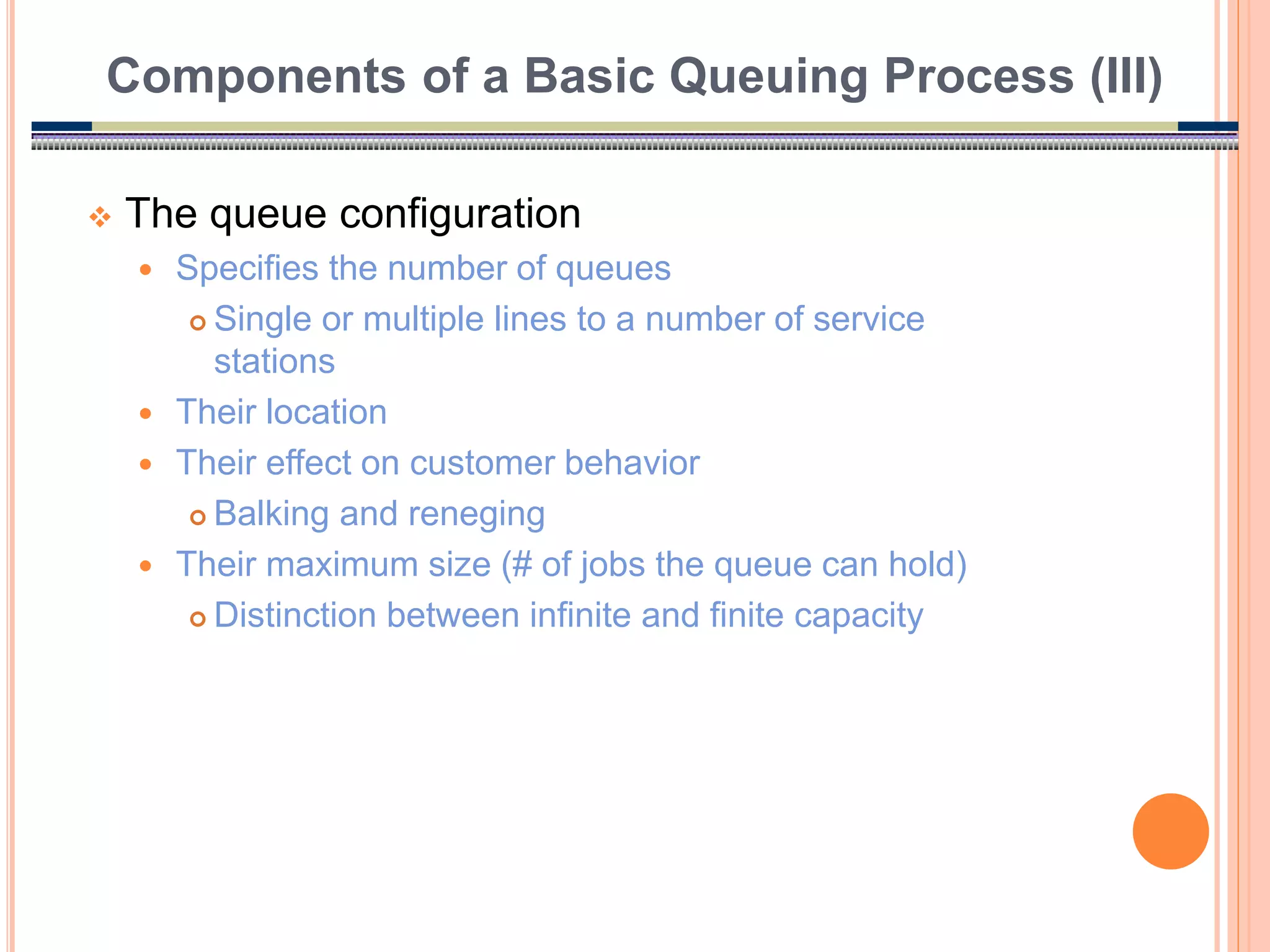
 The queue configuration
 Specifies the number of queues
 Single or multiple lines to a number of service
stations
 Their location
 Their effect on customer behavior
 Balking and reneging
 Their maximum size (# of jobs the queue can hold)
 Distinction between infinite and finite capacity
Components of a Basic Queuing Process (III)

10. 9
 The Service Mechanism
 Can involve one or several service facilities with one or several
parallel service channels (servers) - Specification is required
 The service provided by a server is characterized by its service time
 Specification is required and typically involves data gathering and
statistical analysis.
 Most analytical queuing models are based on the assumption of
exponentially distributed service times, with some generalizations.
 The queue discipline
 Specifies the order by which jobs in the queue are being served.
 Most commonly used principle is FIFO.
 Other rules are, for example, LIFO, SPT, EDD…
 Can entail prioritization based on customer type.
Components of a Basic Queuing Process (IV)

11. 11
A Commonly Seen Queuing Model (I)
C C C … C
Customers (C)
C S = Server
C S
•
•
•
C S
Customer =C
The Queuing System
The Queue
The Service Facility

12. 12
 Service times as well as inter arrival times are assumed
independent and identically distributed
 If not otherwise specified
 Commonly used notation principle: (a/b/c):(d/e/f)
 a = The inter arrival time distribution
 b = The service time distribution
 c = The number of parallel servers
 d= Queue discipline
 e = maximum number (finite/infinite) allowed in the system
 f = size of the calling source(finite/infinite)
 Commonly used distributions
 M = Markovian (exponential/possion) –arrivals or departurs
distribution Memoryless
 D = Deterministic distribution
 G = General distribution
 Example: M/M/c
 Queuing system with exponentially distributed service and inter-
arrival times and c servers
A Commonly Seen Queuing Model (II)

13. 14
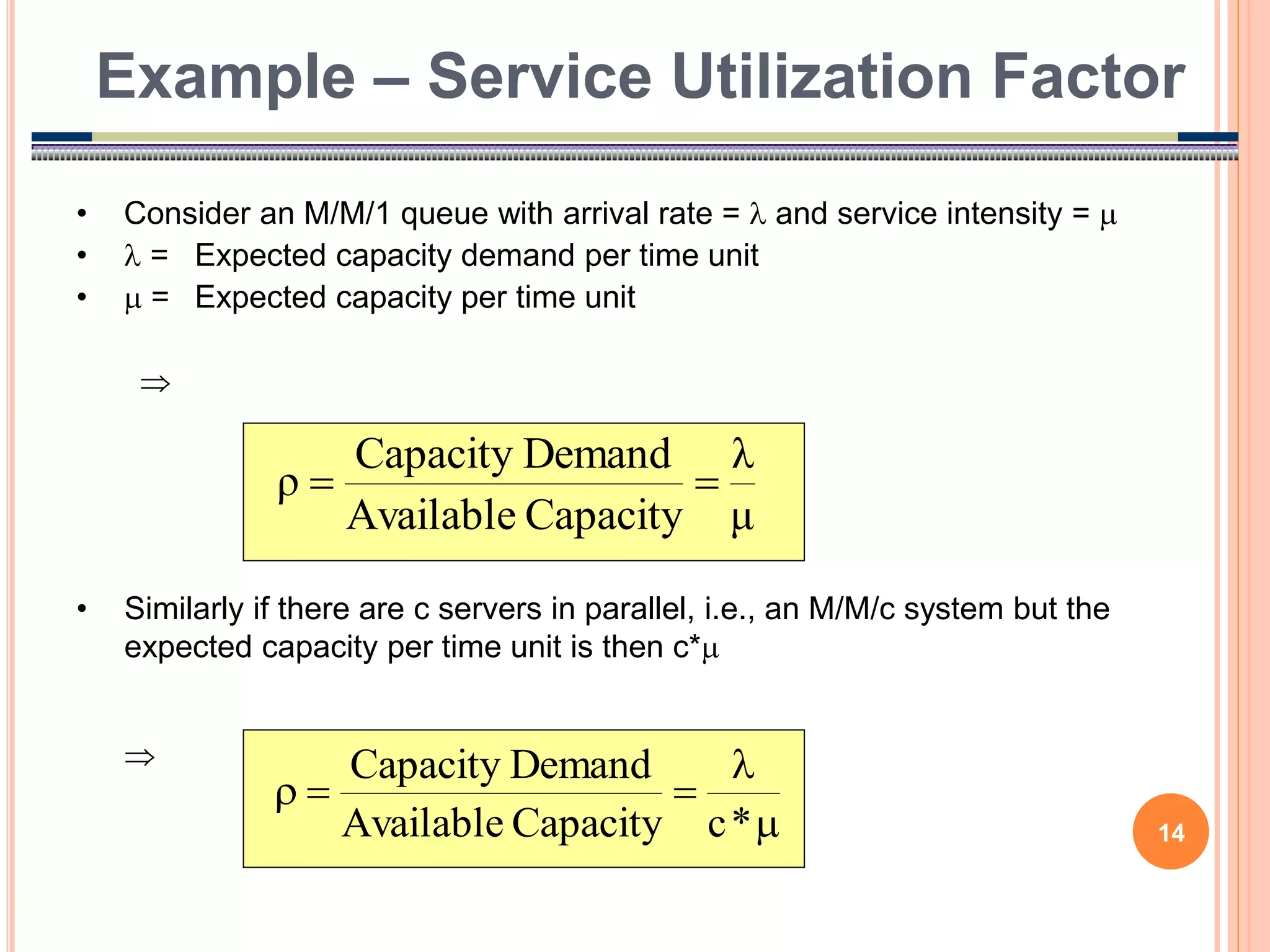
Example – Service Utilization Factor
• Consider an M/M/1 queue with arrival rate =  and service intensity = 
•  = Expected capacity demand per time unit
•  = Expected capacity per time unit

μ
λ
Capacity
Available
Demand
Capacity
ρ 






*
c
Capacity
Available
Demand
Capacity
• Similarly if there are c servers in parallel, i.e., an M/M/c system but the
expected capacity per time unit is then c*


14. 13
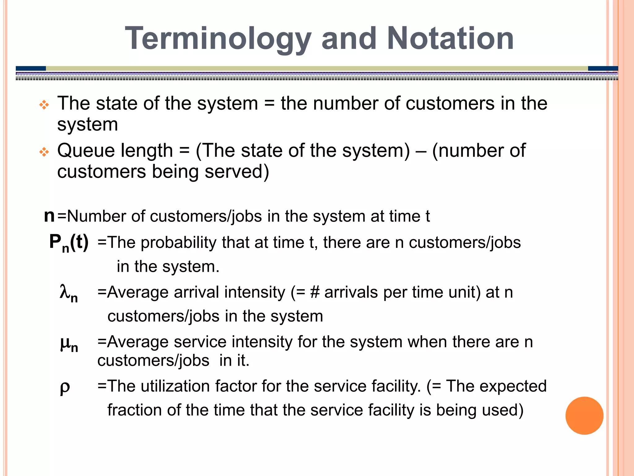
 The state of the system = the number of customers in the
system
 Queue length = (The state of the system) – (number of
customers being served)
n=Number of customers/jobs in the system at time t
Pn(t) =The probability that at time t, there are n customers/jobs
in the system.
n =Average arrival intensity (= # arrivals per time unit) at n
customers/jobs in the system
n =Average service intensity for the system when there are n
customers/jobs in it.
 =The utilization factor for the service facility. (= The expected
fraction of the time that the service facility is being used)
Terminology and Notation

15. 15
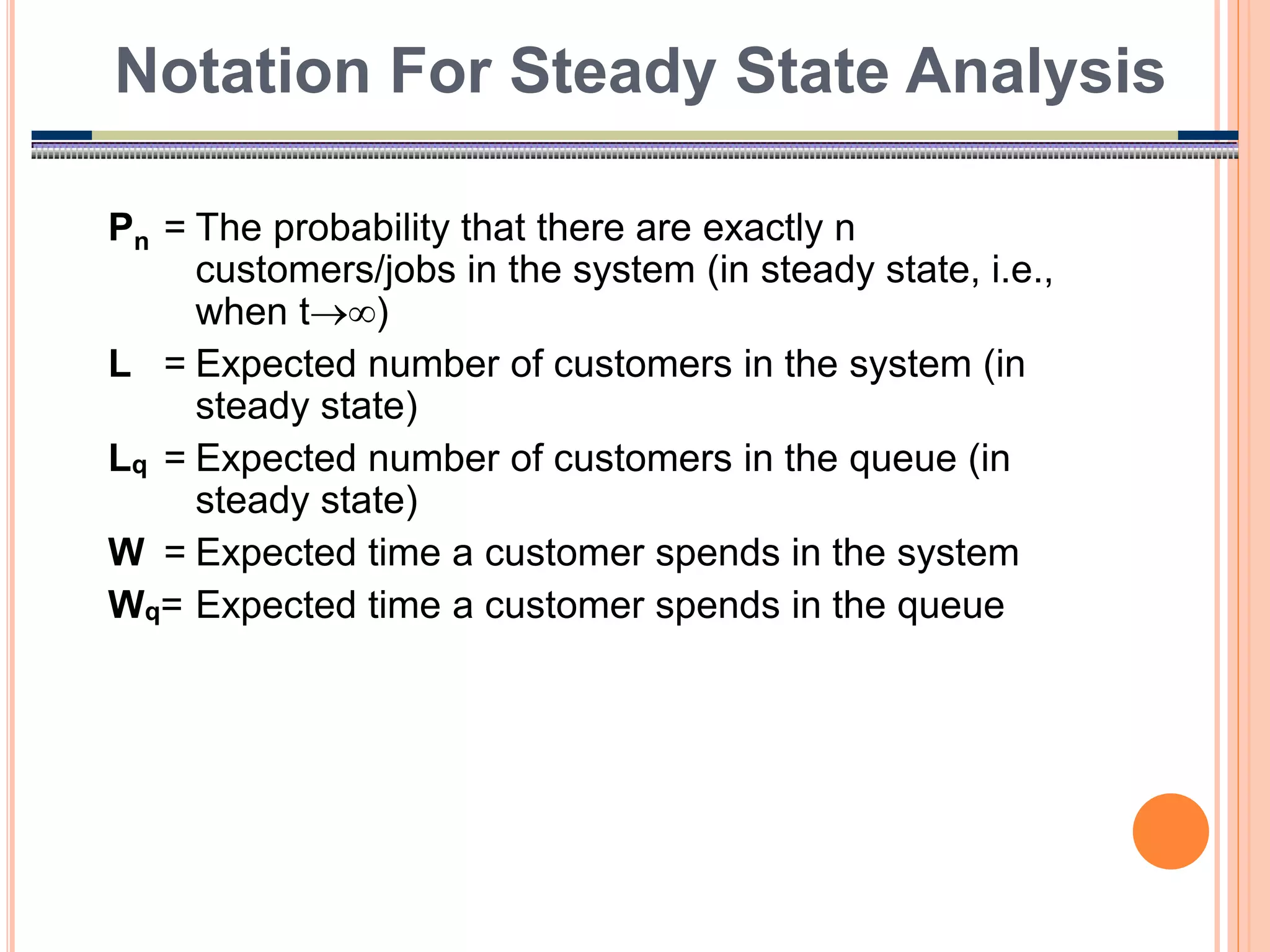
Pn = The probability that there are exactly n
customers/jobs in the system (in steady state, i.e.,
when t)
L = Expected number of customers in the system (in
steady state)
Lq = Expected number of customers in the queue (in
steady state)
W = Expected time a customer spends in the system
Wq= Expected time a customer spends in the queue
Notation For Steady State Analysis

16. 16
 Assume that n =  and n =  for all n
 Assume that n is dependent on n
Little’s Formula
W
L 
 q
q W
L 

W
L 
 q
q W
L 







0
n
n
n
P
Let

17. 17
Assumptions - the Basic Queuing Process
 Infinite Calling Populations
 Independence between arrivals
 The arrival process is Poisson with an expected arrival rate 
 Independent of the number of customers currently in the system
 The queue configuration is a single queue with possibly
infinite length
 No reneging or balking
 The queue discipline is FIFO
 The service mechanism consists of a single server with
exponentially distributed service times
  = expected service rate when the server is busy
The M/M/1 - model

18. 18
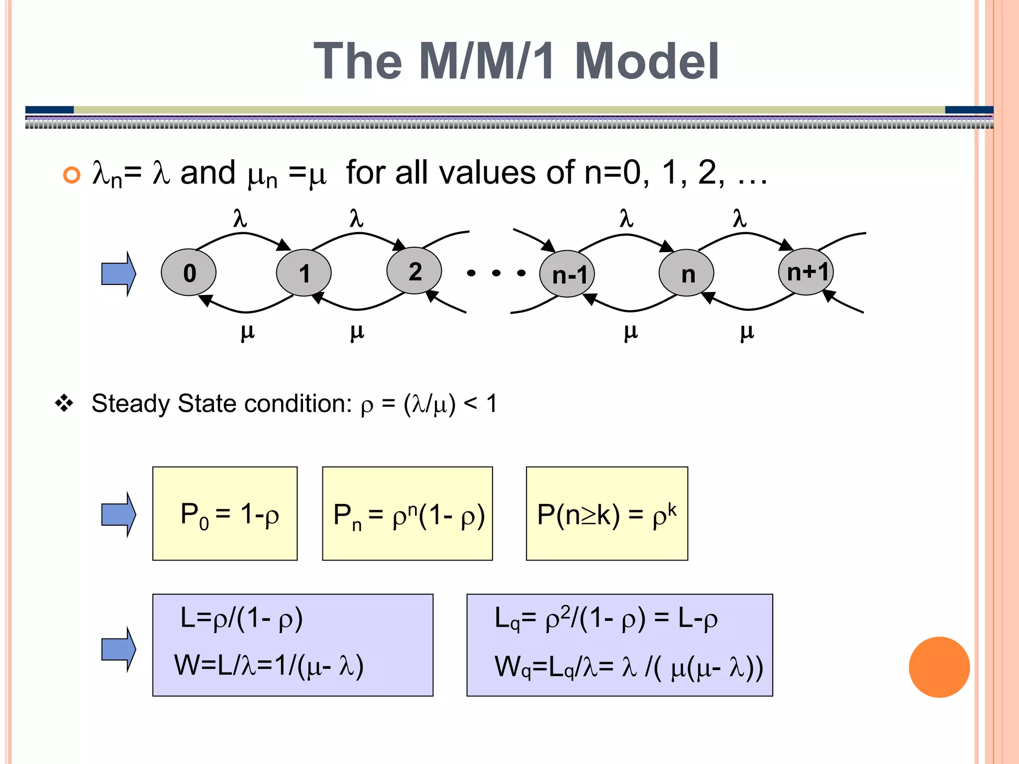
 n=  and n = for all values of n=0, 1, 2, …
The M/M/1 Model
0 
   
   
1 n
n-1
2 n+1
L=/(1- ) Lq= 2/(1- ) = L-
W=L/=1/(- ) Wq=Lq/=  /( (- ))
 Steady State condition:  = (/) < 1
Pn = n(1- )
P0 = 1- P(nk) = k

19. 19
 Situation
 Patients arrive according to a Poisson process with
intensity  ( the time between arrivals is exp()
distributed.
 The service time (the doctor’s examination and treatment
time of a patient) follows an exponential distribution with
mean 1/ (=exp() distributed)
 The SMS can be modeled as an M/M/c system where
c=the number of doctors
Example – SMS Hospital
 Data gathering
  = 2 patients per hour
  = 3 patients per hour
 Questions
– Should the capacity be increased from 1 to 2 doctors?
– How are the characteristics of the system (, Wq, W, Lq and
L) affected by an increase in service capacity?

20. 20
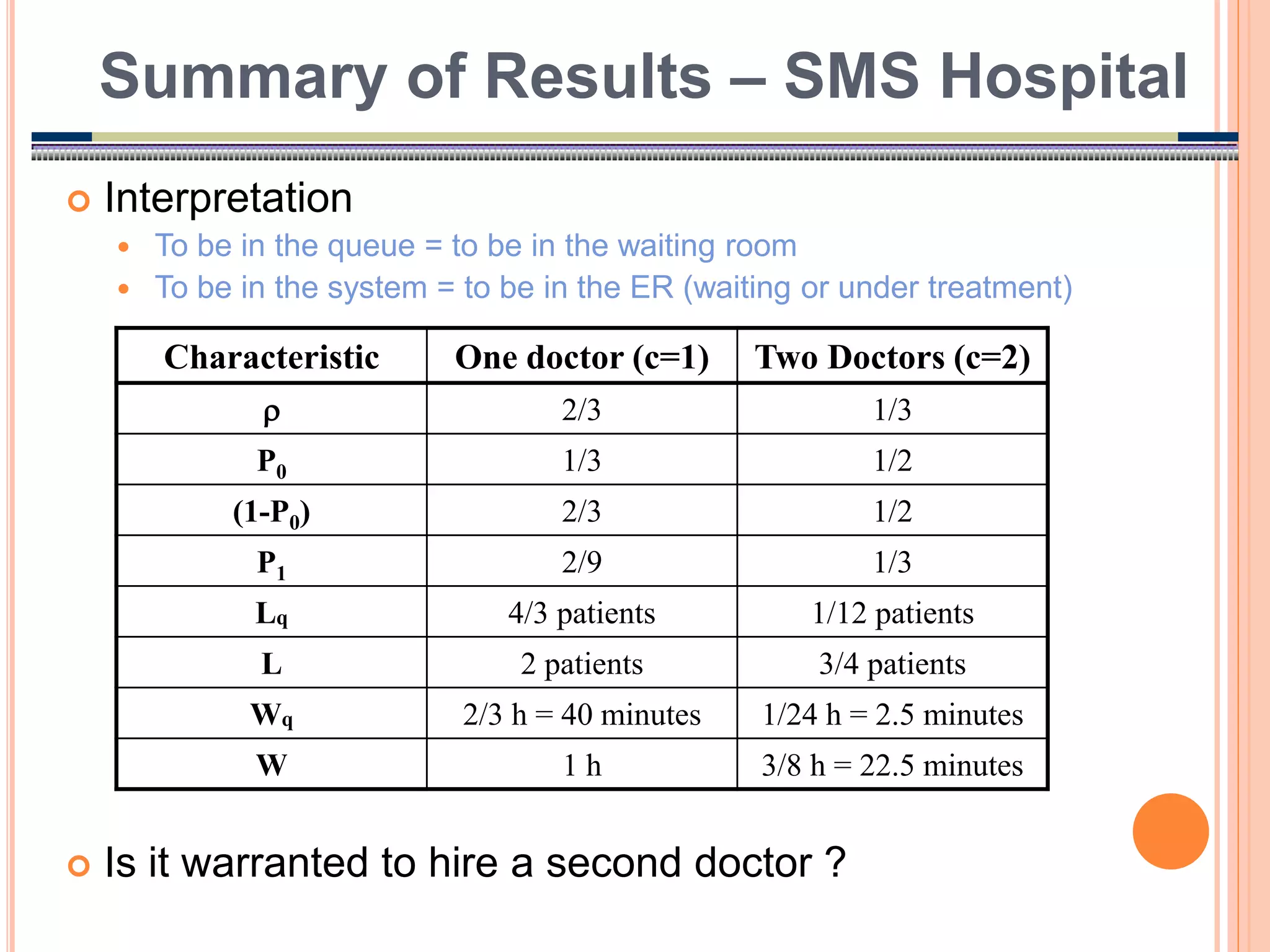
 Interpretation
 To be in the queue = to be in the waiting room
 To be in the system = to be in the ER (waiting or under treatment)
 Is it warranted to hire a second doctor ?
Summary of Results – SMS Hospital
Characteristic One doctor (c=1) Two Doctors (c=2)
 2/3 1/3
P0 1/3 1/2
(1-P0) 2/3 1/2
P1 2/9 1/3
Lq 4/3 patients 1/12 patients
L 2 patients 3/4 patients
Wq 2/3 h = 40 minutes 1/24 h = 2.5 minutes
W 1 h 3/8 h = 22.5 minutes

21. 21
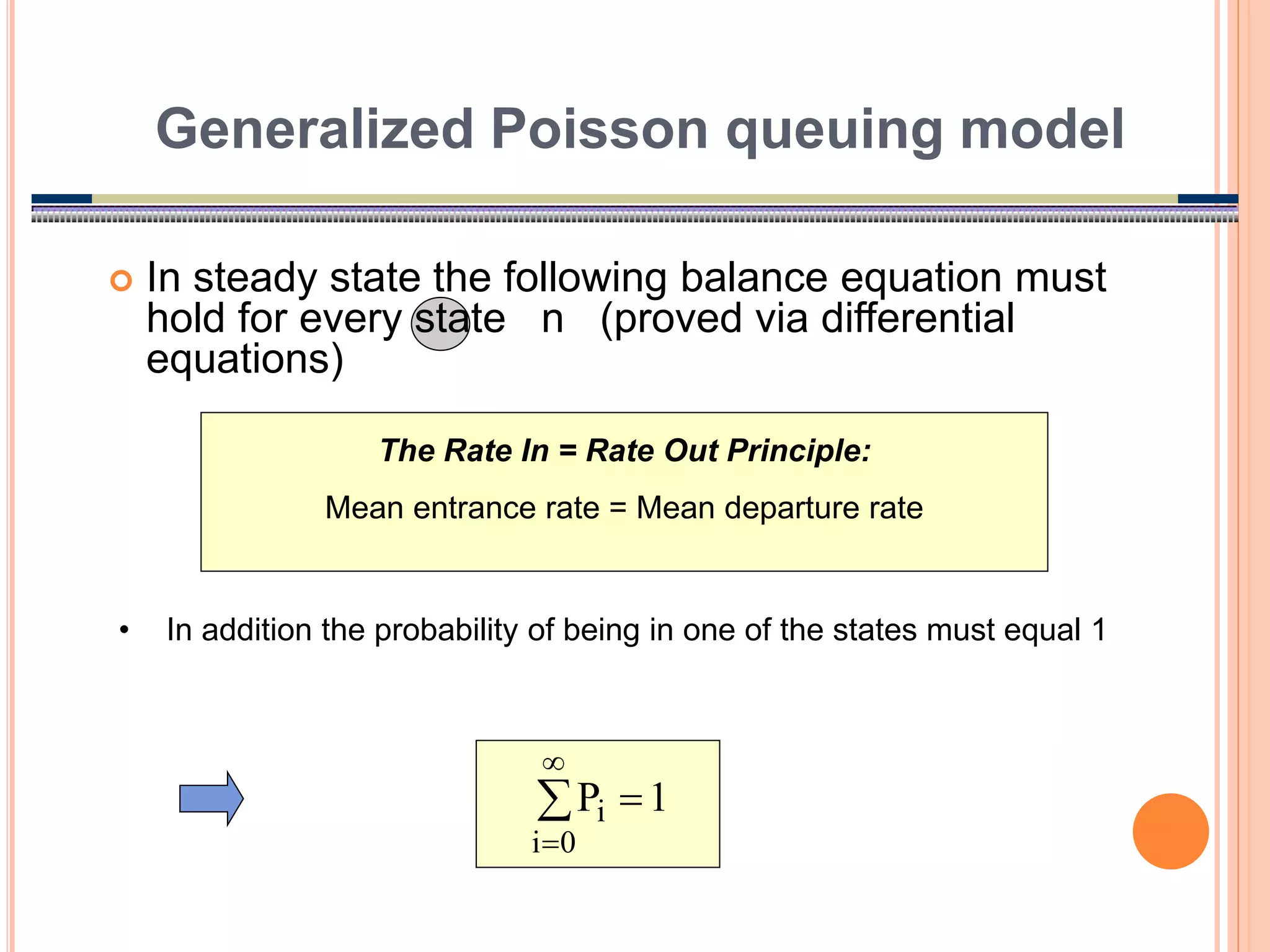
 In steady state the following balance equation must
hold for every state n (proved via differential
equations)
Generalized Poisson queuing model
The Rate In = Rate Out Principle:
Mean entrance rate = Mean departure rate




0
i
i 1
P
• In addition the probability of being in one of the states must equal 1

22. 22
0
0
1
1 P
P 


State Balance Equation
0
1
n
1
1
1
1
2
2
0
0 P
P
P
P 







n
n
n
1
n
1
n
1
n
1
n P
)
(
P
P 





 



Generalized Poisson queuing model
0
1
0
1 P
P




1
2
1
2 P
P



1
n
n
1
n
n P
P 




 
1
1
P
P
:
ion
Normalizat
0
i 3
2
1
2
1
0
2
1
1
0
1
0
0
i 



























C0 C2

23. 23
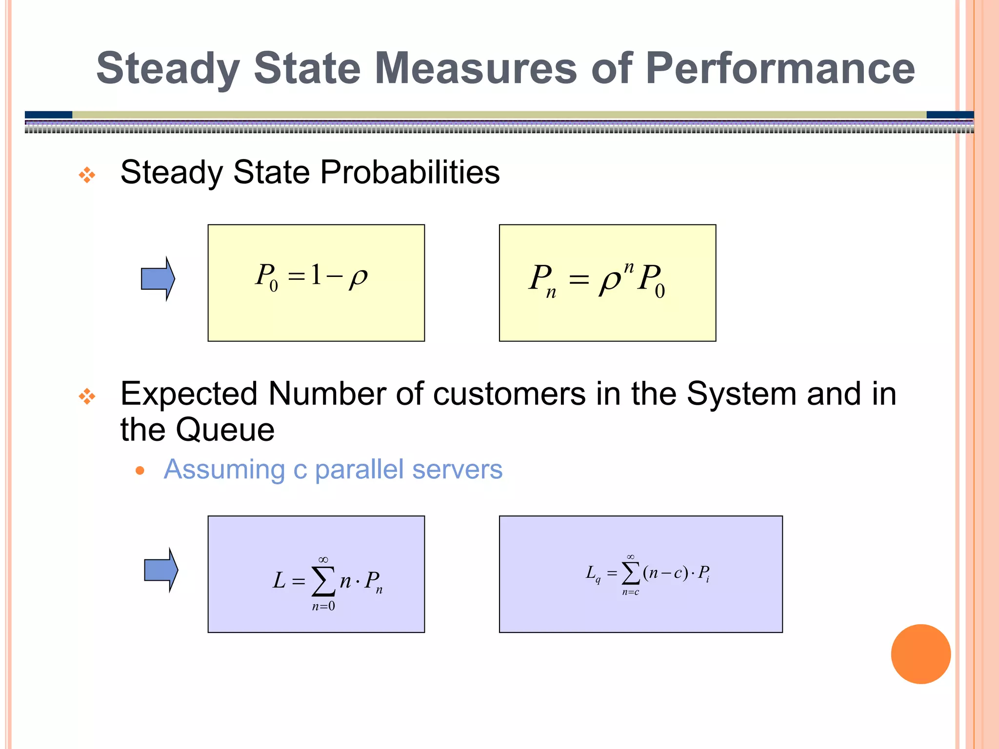
 Steady State Probabilities
 Expected Number of customers in the System and in
the Queue
 Assuming c parallel servers
Steady State Measures of Performance


1
0
P 0
P
P n
n 






0
n
n
P
n
L 





c
n
i
q P
c
n
L )
(

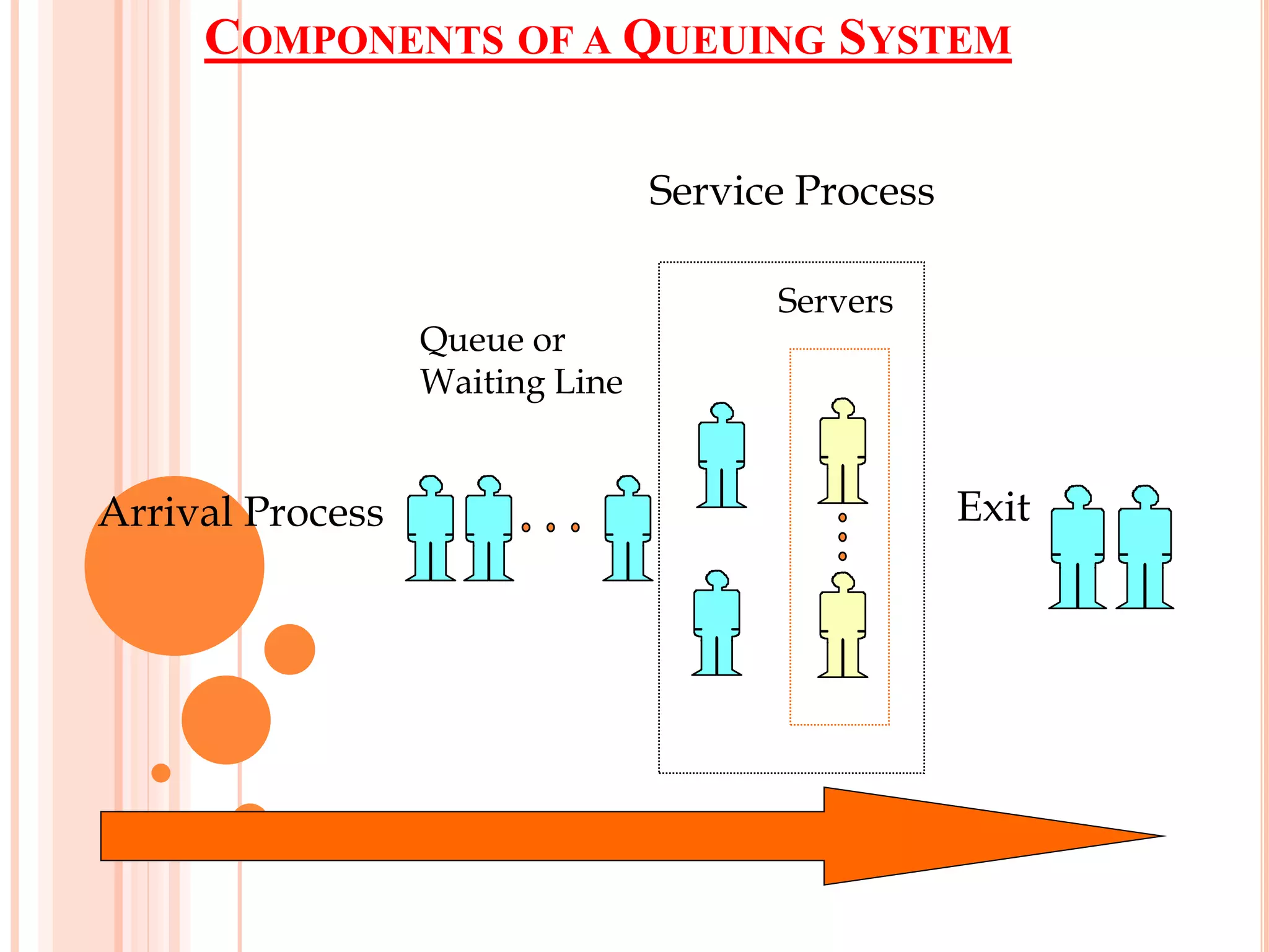
24. COMPONENTS OF A QUEUING SYSTEM
Arrival Process
Servers
Queue or
Waiting Line
Service Process
Exit

25. 25
The M/M/c Model (I)
1
c
1
c
0
n
n
0
)
c
/(
(
1
1
!
c
)
/
(
!
n
)
/
(
P




















 



















,
2
c
,
1
c
n
for
P
c
!
c
)
/
(
c
,
,
2
,
1
n
for
P
!
n
)
/
(
P
0
c
n
n
0
n
n
0 
   
 2 (c-1) c
1 c
c-2
2 c+1

c
c-1
(c-2)
• Generalization of the M/M/1 model
– Allows for c identical servers working independently from each
other
Steady State
Condition:
=(/c)<1

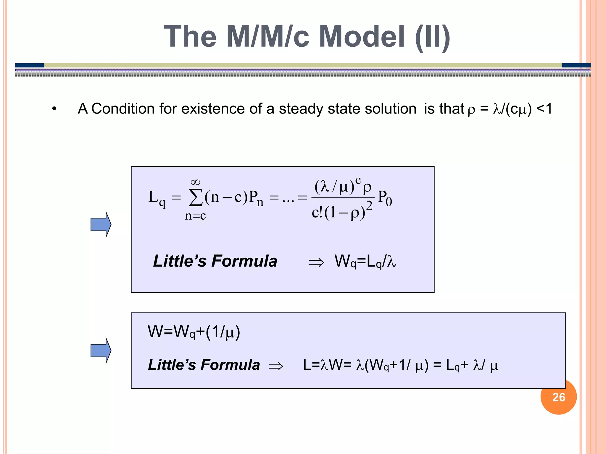
26. 26
W=Wq+(1/)
Little’s Formula  Wq=Lq/
The M/M/c Model (II)
0
2
c
c
n
n
q P
)
1
(
!
c
)
/
(
...
P
)
c
n
(
L








 


• A Condition for existence of a steady state solution is that  = /(c) <1
Little’s Formula  L=W= (Wq+1/ ) = Lq+ / 

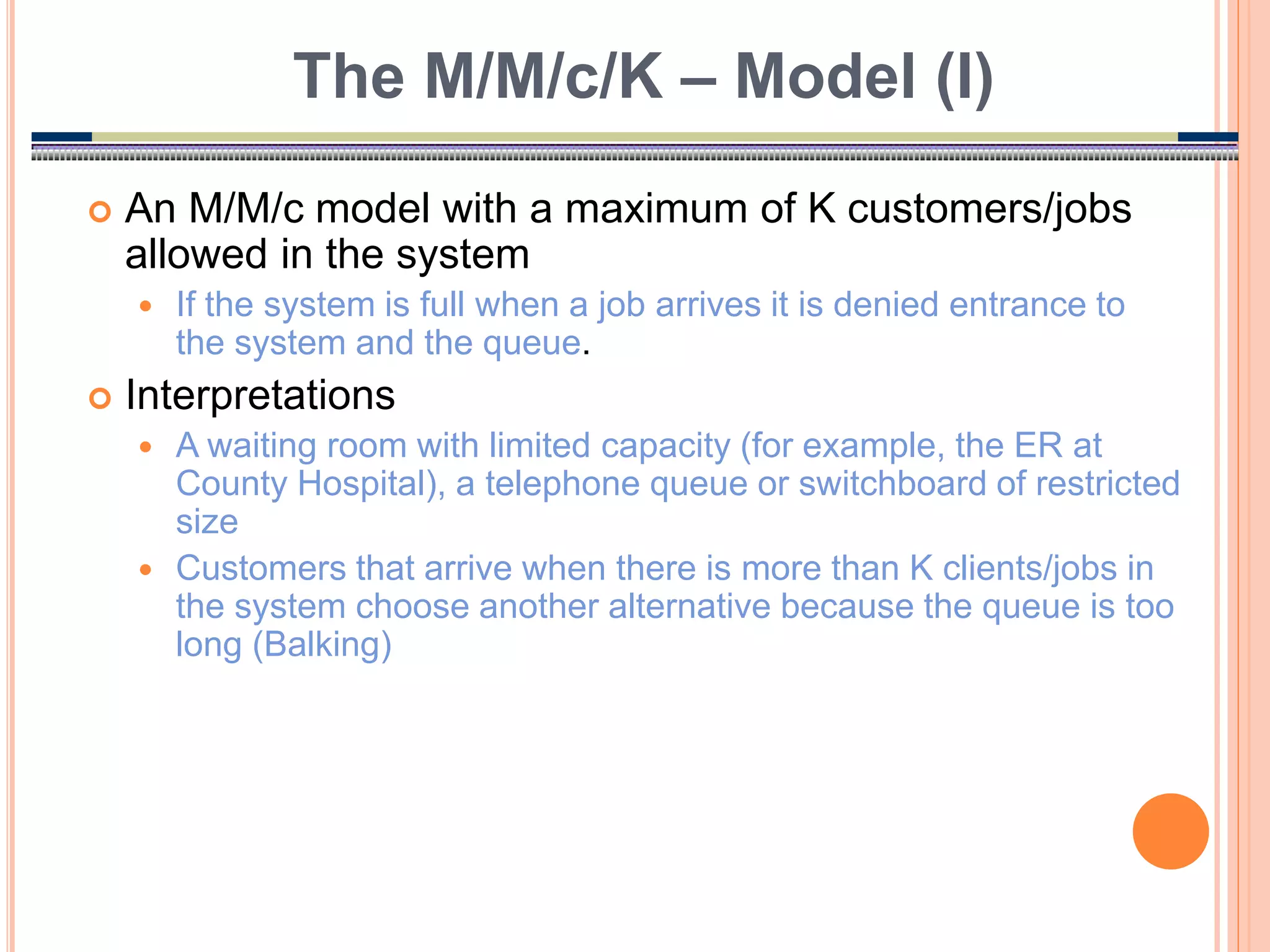
27. 27
 An M/M/c model with a maximum of K customers/jobs
allowed in the system
 If the system is full when a job arrives it is denied entrance to
the system and the queue.
 Interpretations
 A waiting room with limited capacity (for example, the ER at
County Hospital), a telephone queue or switchboard of restricted
size
 Customers that arrive when there is more than K clients/jobs in
the system choose another alternative because the queue is too
long (Balking)
The M/M/c/K – Model (I)

28. 28
 The state diagram has exactly K states provided that
c<K
 The general expressions for the steady state
probabilities, waiting times, queue lengths etc. are
obtained through the balance equations as before
(Rate In = Rate Out; for every state)
The M/M/c/K – Model (II)
0 
   
 2 (c-1) c
1 K-1
c-1
2 K
c 
c
c
 
 
3

29. 29
 An M/M/c model with limited calling population, i.e., N
clients
 A common application: Machine maintenance
 c service technicians is responsible for keeping N service
stations (machines) running, that is, to repair them as soon as
they break
 Customer/job arrivals = machine breakdowns
 Note, the maximum number of clients in the system = N
 Assume that (N-n) machines are operating and the time
until breakdown for each machine i, Ti, is exponentially
distributed (Tiexp()). If U = the time until the next
breakdown
 U = Min{T1, T2, …, TN-n}  Uexp((N-n))).
The M/M/c//N – Model (I)

30. 30
• The State Diagram (c service technicians and N machines)
–  = Arrival intensity per operating machine
–  = The service intensity for a service technician
• General expressions for this queuing model can be obtained from the
balance equations as before
The M/M/c//N – Model (II)
0 
N (N-1) (N-(c-1)) 
 2 (c-1) c
1 N-1
c-1
2 N
c 
c
3

31. Reference:-
1. Operations research: an introduction
By:- Hamdy A. Taha
2 . Operations research
By:-P.Sankar Iyar