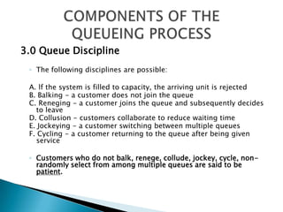
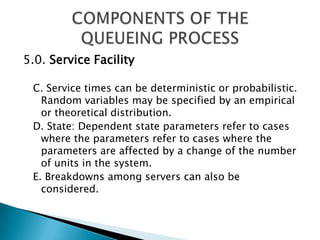
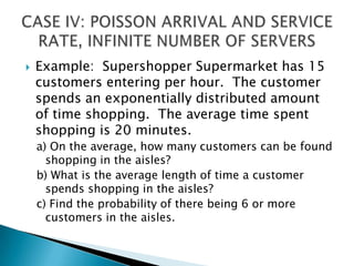
![Notations: λc = effective mean arrival rate λ = λc if queue is infinite λe = λ - [expected number who balk if the queue is finite] W = expected waiting time of a customer in the system Wq = expected waiting time of a customer in the queue L = expected no. of customers in the system Lq = expected number of customers in the queue Po = probability of no customers in the system Pn = probability of n customers in the system ρ = traffic intensity= λ/μρc= effective traffic intensity= λe/μCLASSIFICATIONS OF MODELS AND SOLUTIONS](https://image.slidesharecdn.com/queueingtheory-110227225225-phpapp02/85/Queueing-theory-15-320.jpg)
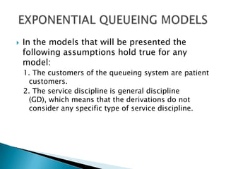
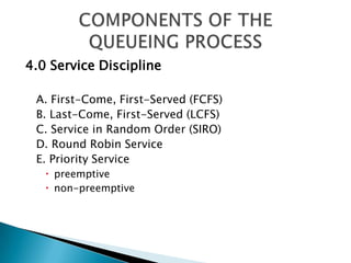
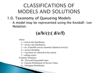
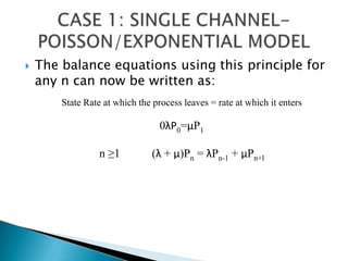
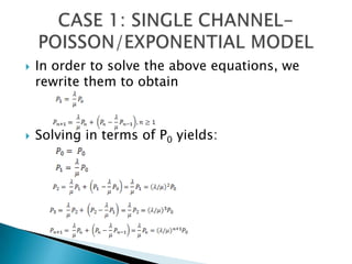
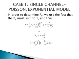
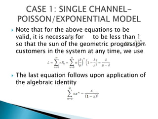
![SINGLE CHANNEL-POISSON/EXPONENTIAL MODEL [(M/M/1):(GD/ α /α)] Characteristics: 1. Input population is infinite. 2. Arrival rate has a Poisson Distribution 3. There is only one server. 4. Service time is exponentially distributed with mean1/μ. [λ<μ] 5. System capacity is infinite. .6. Balking and reneging are not allowed. CASE 1: SINGLE CHANNEL-POISSON/EXPONENTIAL MODEL](https://image.slidesharecdn.com/queueingtheory-110227225225-phpapp02/85/Queueing-theory-19-320.jpg)
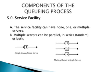
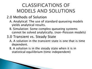
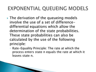
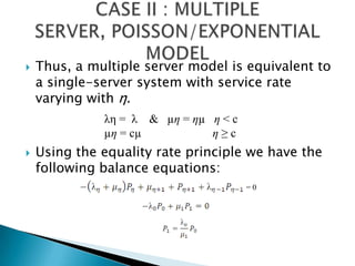
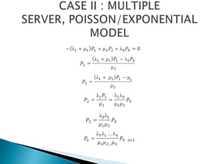
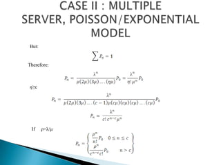
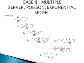
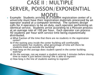
![MULTIPLE SERVER, POISSON/EXPONENTIAL MODEL [(M/M/C):(GD/∞/∞ )] The assumptions of Case II are the same as Case 1 except that the number of service channels is more than one. For this case, the service rate of the system is given by: CASE II : MULTIPLE SERVER, POISSON/EXPONENTIAL MODEL cµ η ≥ cηµ η < c](https://image.slidesharecdn.com/queueingtheory-110227225225-phpapp02/85/Queueing-theory-29-320.jpg)

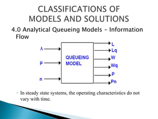
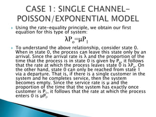
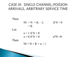
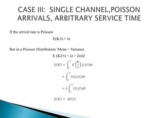
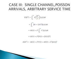
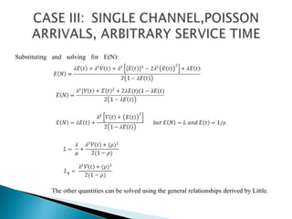
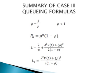
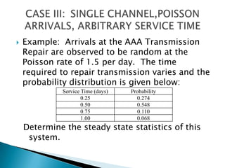
![SINGLE CHANNEL,POISSON ARRIVALS, ARBITRARY SERVICE TIME : Pollaczek - Khintchine Formula [(M/G/l): (GD/∞/∞)] This case is similar to Case 1 except that the service rate distribution is arbitrary. Let: N = no. of units in the queueing system immediately after a unit departs T = the time needed to service the unit that follows the one departing (unit 1) at the beginning of the time count. K= no. of new arrivals units the system during the time needed to service the unit that follows the one departing (unit 1) Nl = no. of units left in the system when the unit (1) departs CASE III: SINGLE CHANNEL,POISSON ARRIVALS, ARBITRARY SERVICE TIME](https://image.slidesharecdn.com/queueingtheory-110227225225-phpapp02/85/Queueing-theory-37-320.jpg)
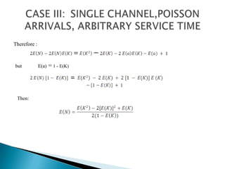
![CASE III: SINGLE CHANNEL,POISSON ARRIVALS, ARBITRARY SERVICE TIMEIn a steady state system: ~. E(N) = E( ) E () =E[ ] ) = E (E (a) = -E (K) + 1 =a*N= 0 =Since a = 0 or 1: But](https://image.slidesharecdn.com/queueingtheory-110227225225-phpapp02/85/Queueing-theory-39-320.jpg)
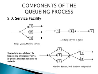
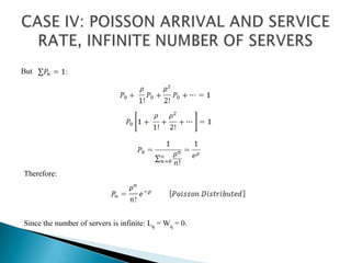
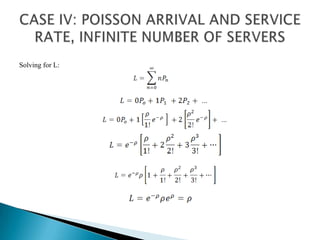
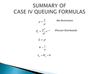
![POISSON ARRIVAL AND SERVICE RATE, INFINITE NUMBER OF SERVERS: Self-Service Model [(M/M/∞): (GD/∞/∞)]Consider a multiple server system. The equivalent single server system if the number of servers is infinite would be:From the multiple server system:CASE IV: POISSON ARRIVAL AND SERVICE RATE, INFINITE NUMBER OF SERVERS](https://image.slidesharecdn.com/queueingtheory-110227225225-phpapp02/85/Queueing-theory-46-320.jpg)
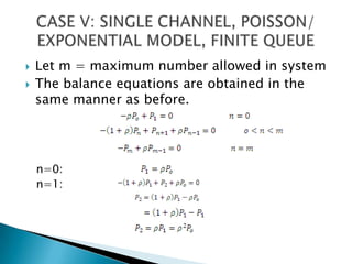
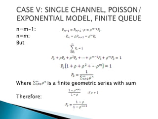
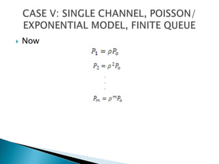
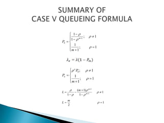
![SINGLE CHANNEL, POISSON/EXPONENTIAL MODEL, FINITE QUEUE [(M/M/1) : (GD/m/∞)]This case is similar to Case 1 except that the queue is finite, i.e., when the total number of customers in the system reaches the allowable limit, all arrivals balk.CASE V: SINGLE CHANNEL, POISSON/ EXPONENTIAL MODEL, FINITE QUEUE](https://image.slidesharecdn.com/queueingtheory-110227225225-phpapp02/85/Queueing-theory-51-320.jpg)
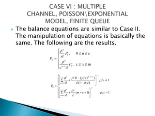
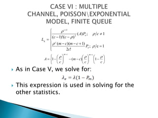
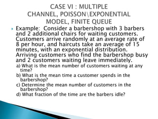
![MULTIPLE CHANNEL, POISSON\ EXPONENTIAL MODEL, FINITE QUEUE [(M/M/c):(GD/m/∞)]This case is an extension of Case V. We assume that the number of service channels is more than one. For this system: CASE VI : MULTIPLE CHANNEL, POISSON\EXPONENTIAL MODEL, FINITE QUEUE](https://image.slidesharecdn.com/queueingtheory-110227225225-phpapp02/85/Queueing-theory-57-320.jpg)
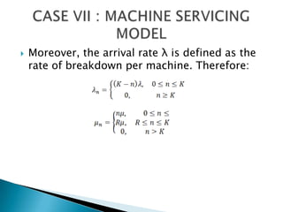
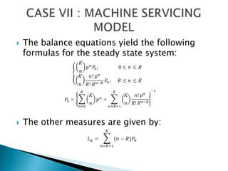
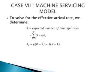
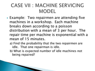
![MACHINE SERVICING MODEL [(M/M/R):(GD/K/K)]This model assumes that R repairmen are available for servicing a total of K machines. Since a broken machine cannot generate new calls while in service, this model is an example of finite calling source. This model can be treated as a special case of the single server, infinite queue model. CASE VII : MACHINE SERVICING MODEL](https://image.slidesharecdn.com/queueingtheory-110227225225-phpapp02/85/Queueing-theory-61-320.jpg)
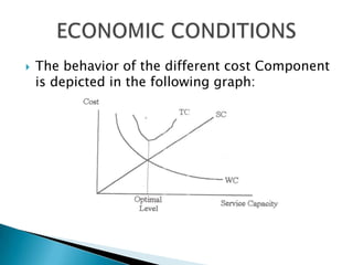

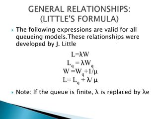
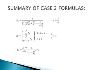
Queueing theory studies waiting line systems where customers arrive for service but servers have limited capacity. This document outlines components of queueing models including: arrival processes, queue configurations, service disciplines, service facilities, and analytical solutions. Key points are that customers wait in queues when demand exceeds server capacity, and queueing formulas provide expected wait times and number of customers in the system based on arrival and service rates.