Queuing theory is the mathematical study of waiting lines in systems like traffic networks, telephone systems, and more. It examines elements like arrival and service rates to predict system performance. The document outlines key concepts in queuing systems such as customers, servers, applications, and components like arrival processes, queue configuration, service disciplines, and service facilities. Special delay studies models are also discussed, including models for merging delays and peak flow delays.

1. Queuing Theory
Prepared by:
Pranav Mishra
Indian Institute of Technology Kharagpur
Indian Institute of Technology Kharagpur

2. Queuing Theory
•Queuing theory is the mathematics of waiting lines.
•A queue forms whenever existing demand exceeds the existing capacity of
service facility.
•It is extremely useful in predicting and evaluating system performance.
Queuing system
Customer
input output
Server
Queue
Key elements of queuing system
a) Customers : Refers to anything that arrives at facility and
requires service
b) Servers: Refers to any resource that provides the
requested service
Indian Institute of Technology Kharagpur

3. pplications of queuing theory
•Telecommunications
•Traffic control
•Layout of manufacturing systems
•Airport traffic
•Ticket sales counter, etc.
Examples: System Customers Server
Reception desk People Receptionist
Hospital Patients Nurses
Airport Airplanes Runway
Road network Cars Traffic light
Grocery Shoppers Checkout station
Computer Jobs CPU, disk, CD
Indian Institute of Technology Kharagpur

4. Components of a queuing system process
Arrivals Service Exit the system
Population of from the Queue facility
dirty cars general (waiting line)
population …
Dave’s
Car Wash
enter exit
Arrivals to the system In the system Exit the system
2) Queue 4) Service discipline
1) Arrival process
configuration
5) Service facility
3) Queue discipline
Indian Institute of Technology Kharagpur

5. Components of a queuing system process
1) Arrival process
•The source may be,
•single or multiple.
•Size of the population may be,
•finite or infinite.
•Arrival may be single or bulk.
•Control on arrival may be,
•Total control.
•Partial control.
•No control
•Statistical distribution of arrivals may be,
•Deterministic,
•Probabilistic.
Indian Institute of Technology Kharagpur

6. Components of a queuing system process
2) Queue configuration
•The queue configuration refers to,
• number of queues in the system,
•Their spatial consideration,
•Their relationship with server.
•A queue may be single or multiple queue.
•A queuing system may impose restriction on the maximum number of units
allowed.
3) Queue discipline
•If the system is filled to capacity, arriving unit is not allowed to join the queue.
•Balking – A customer does not join the queue.
•Reneging – A customer joins the queue and subsequently decides to leave.
•Collusion – Customers collaborate to reduce the waiting time.
•Jockeying – A customer switching between multiple queues.
•Cycling – A customer returning to the queue after being served.
•A queue may be single or multiple queue.
Indian Institute of Technology Kharagpur

7. Components of a queuing system process
4) Service discipline
•First In First Out (FIFO) a.k.a First Come First Serve (FCFS)
•Last In First Out (LIFO) a.k.a Last Come First Served (LCFS).
•Service In Random Order (SIRO).
•Priority Service
•Preemptive
•Non-preemptive
5) Service facility
•Single queue single server
Service Departures
Arrivals after service
facility
Queue
Indian Institute of Technology Kharagpur

8. Components of a queuing system process
5) Service facility
•Single queue multiple server
Service
facility
Channel 1
Queue
Service Departures
Arrivals facility
after service
Channel 2
Service
facility
Channel 3
Indian Institute of Technology Kharagpur

9. Components of a queuing system process
5) Service facility
•Multiple queue multiple server
Customers
Arrivals Queues Service station
leave
Indian Institute of Technology Kharagpur

10. Components of a queuing system process
5) Service facility
•Multiple server in series
Service station 1 Service station 2
Arrivals
Phase 1 Phase 2
Queues Queues
Customers
leave
Indian Institute of Technology Kharagpur

11. Queuing models : some basic relationships
λ = Mean number of arrivals per time period
µ = Mean number of units served per time period
Assumptions:
• If λ > µ, then waiting line shall be formed and increased indefinitely and
service system would fail ultimately.
• If λ < µ, there shall be no waiting line.
Average number of units (customers) in the system (waiting and being served)
= λ/ (µ - λ)
Average time a unit spends in the system (waiting time plus service time)
= 1/ (µ - λ)
Indian Institute of Technology Kharagpur

12. Queuing models : some basic relationships
Average number of units waiting in the queue
= λ 2/ µ(µ - λ)
Average time a unit spends waiting in the queue
= λ/ µ(µ - λ)
Intensity or utilization factor
= λ/ µ
Indian Institute of Technology Kharagpur

13. Special Delay studies
a) Merging delays
b) Peak flow delay
c) Parking
a) Merging delays
Merging may be defined as absorption of one group of traffic by another.
Oliver & Bisbee postulated that minor stream queue length are function of
major street flow rates.
This model assumes that:
•A gap of at-least T is required to enter the major stream.
•Only one entry is permitted through one acceptable gap.
•Entries occur just after passing of vehicles, that signals beginning of gap of
acceptable size.
Indian Institute of Technology Kharagpur

14. Special Delay studies
• Appearance of gap in major stream is not affected by queue in minor
stream; and,
• Arrivals into the minor stream queue are Poisson
Average number of vehicles in minor stream queue E(n)
Where,
qa = minor stream flow,
qb = major stream flow,
T = minimum acceptable gap
Indian Institute of Technology Kharagpur

15. Special Delay studies
This model works particularly better for the situation,
• Where major stream flow rate is high, and
• Vehicles in minor stream queue are served on FIFO basis, with the
appearance of a minimum acceptable gap T.
HO formulated a model to predict the amount of time required to clear two
joining traffic streams through a merging point.
This model assumes that:
•Merging is permitted only at merging point.
•Vehicles are served in FIFO basis.
Indian Institute of Technology Kharagpur

16. Special Delay studies
The total time required for n1 and n2 vehicles to pass through the merging
point is,
Where,
hi = i’th time gap on major road,
to = time required for a vehicle to merge into through traffic, assuming all
vehicles take same time to merge.
α = number of vehicle that merge into i’th gap.
n1 = number of vehicle in major road,
n2 = number of vehicle waiting to merge
Indian Institute of Technology Kharagpur

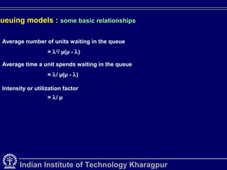
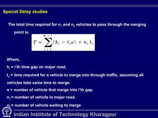
17. Special Delay studies
b) Peak flow delay
• If traffic demand exceeds the capacity, there is a continuous buildup of
traffic.
• Mean service rate exceeds the mean rate of arrival.
• Expected number of vehicle ‘n’, waiting in the system at any time ‘t’ can be
represented as E[n(t)] and will grow indefinitely as ‘t’ increases.
E[n(t)] = E(n) + λ(t) - μ(t)
• E(n) = expected number of vehicles in system with initial traffic intensity ρo,
where, ρo <1
• λ = mean arrival rate and, μ = mean service rate
Indian Institute of Technology Kharagpur

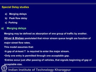
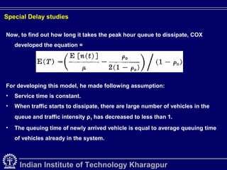
18. Special Delay studies
• Now, say traffic intensity ρo increases to ρ1 , where ρ1 >1
• Therefore, ρ1 = λ / μ [ initial λ0 increases to λ]
or λ = μ . ρ1
• So, E[n(t)] = E(n) - μ . ρ1 (t) - μ(t)
E[n(t)] = E(n) + (ρ1 - 1) μ . t
Or, E[n(t)] = ρ0 /(1 - ρ0 ) + (ρ1 - 1) μ . t
• When, service rate (μ) is constant,
E[n(t)] = (1/2) λ0 2 / μ(μ - λ0 ) + λ0/μ + (ρ1 - 1) μ
Indian Institute of Technology Kharagpur

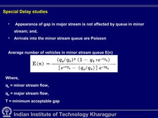
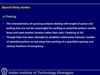
19. Special Delay studies
Numerical example:
• A queue with random arrival rate 1 vehicle per minute and a mean service
time of 45 seconds. In peak period, arrival rate suddenly doubles and this
peak period rate is maintained for 1 hour. Find the average number of
vehicles in the system at the end of peak hour.
Sol. – Given, λ0 = 1, μ = 4/3 Therefore, ρ0 = λ0 / μ = 3/4
In peak period, λ = 2 and μ remains same. So, ρ1 = 3/2
Putting the values in eqn - , E[n(t)] = ρ0 /(1 - ρ0 ) + (ρ1 - 1) μ . t
we get, E[n(60)] = 43
If the service rate μ were constant,
Putting the values in eqn - , E[n(t)] = (1/2) λ0 2 / μ(μ - λ0 ) + λ0/μ + (ρ1 - 1) μ
we get, E[n(60)] = 41.87~ 42
Indian Institute of Technology Kharagpur

20. Special Delay studies
Now, to find out how long it takes the peak hour queue to dissipate, COX
developed the equation =
For developing this model, he made following assumption:
• Service time is constant.
• When traffic starts to dissipate, there are large number of vehicles in the
queue and traffic intensity ρ1 has decreased to less than 1.
• The queuing time of newly arrived vehicle is equal to average queuing time
of vehicles already in the system.
Indian Institute of Technology Kharagpur

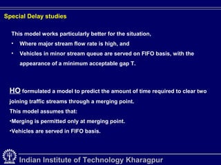
21. Special Delay studies
• For the previous problem, find out the mean time it takes for queue to get
dissipated.
Sol: putting the values in the equation
E (t) = [ E(n)t /μ – ρo / 2(1- ρo ) ] / (1 – ρo )
We get, E(t) = 123 min.
Indian Institute of Technology Kharagpur

22. Special Delay studies
c) Parking
• The characteristics of queuing analysis dealing with length of queue and
waiting time are not too meaningful for parking as potential parkers usually
leave and seek another location rather than wait, if parking is full
• Though there has been attempts to establish relationship between number
of potential parkers turned away from parking of a specified capacity and
various fractions of occupancy.
Indian Institute of Technology Kharagpur