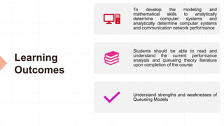
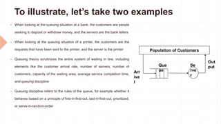
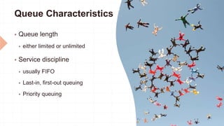
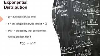
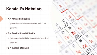
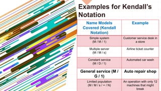
Queing Theory
Dr Renjith V. Ravi Ph. D, FIETE, C. Eng. (IE)
Associate Professor and Head,
Department of Electronics and Communication Engineering
M.E.A Engineering College,
Malappuram District, Kerala, India 679 325
ORCID: 0000-0001-9047-3220
Learning
Outcomes
To develop the modeling and
mathematical skills to analytically
determine computer systems and
analytically determine computer systems
and communication network performance
Students should be able to read and
understand the current performance
analysis and queueing theory literature
upon completion of the course
Understand strengths and weaknesses of
Queueing Models
Introductio
n to
Queuing
Theory
Queuing theory (or queueing theory) refers to the
mathematical study of the formation, function,
and congestion of waiting lines, or queues
At its core, a queuing situation involves two parts
Someone or something that requests a
service—usually referred to as the
customer, job, or request
Someone or something that completes or
delivers the services—usually referred to
as the server
To illustrate, let’s take two examples
 When looking at the queuing situation at a bank, the customers are people
seeking to deposit or withdraw money, and the servers are the bank tellers
 When looking at the queuing situation of a printer, the customers are the
requests that have been sent to the printer, and the server is the printer
 Queuing theory scrutinizes the entire system of waiting in line, including
elements like the customer arrival rate, number of servers, number of
customers, capacity of the waiting area, average service completion time,
and queuing discipline
 Queuing discipline refers to the rules of the queue, for example whether it
behaves based on a principle of first-in-first-out, last-in-first-out, prioritized,
or serve-in-random-order
Population of Customers
Out
put
Se
rve
r
Que
ue
Arr
iva
l
How did queuing theory start?
 Queuing theory was first introduced in the early
20th century by Danish mathematician and
engineer Agner Krarup Erlang
 Erlang worked for the Copenhagen Telephone
Exchange and wanted to analyze and optimize its
operations
 He sought to determine how many circuits were
needed to provide an acceptable level of telephone
service, for people not to be “on hold” for too long
 His mathematical analysis culminated in his 1920
paper “Telephone Waiting Times”, which served as the
foundation of applied queuing theory
 The international unit of telephone traffic is called the
Erlang in his honor
Source: Telephone operators at work
Kendall's
Notation
 In queueing theory, a discipline within the
mathematical theory of probability, Kendall's notation (or
sometimes Kendall notation) is the standard system used to
describe and classify a queueing node.
 D. G. Kendall proposed describing queueing models using
three factors written A/S/c in 1953 where A denotes the time
between arrivals to the queue, S the service time distribution
and c the number of service channels open at the node.
 It has since been extended to A/S/c/K/N/D where K is the
capacity of the queue, N is the size of the population of jobs
to be served, and D is the queueing discipline, assumed first-
in-first-out if omitted.
 When the final three parameters are not specified (e.g. M/M/1
queue), it is assumed K = ∞, N = ∞ and D = FIFO.
Queueing
Discipline
 A network scheduler, also called packet
scheduler, queueing discipline (qdisc) or
queueing algorithm, is an arbiter on a node in a
packet switching communication network.
 It manages the sequence of network packets in
the transmit and receive queues of the protocol
stack and network interface controller.
 There are several network schedulers available
for the different operating systems, that
implement many of the existing network
scheduling algorithms.
Queuing
Disciplines
First-in, first-out queuing
Last-in, first-out queuing
Priority queuing
What are the different types of queuing
systems?
 For example, think of an ATM
 It can serve: one customer at a time; in a first-in-first-out
order; with a randomly-distributed arrival process and
service distribution time; unlimited queue capacity; and
unlimited number of possible customers
 Queuing theory would describe this system as a M/M/1
queue
 Queuing theory calculators out there often require
choosing a queuing system from the Kendall notation
before calculating inputs
Que in front of an ATM
Packet Switching:
queueing delay, loss
 Queuing and loss
 § packets will queue, wait to be
transmitted on link
 § packets can be dropped if memory fills
up
Why is queuing theory
important?
 Waiting in line is a part of everyday life
because as a process it has several important
functions
 Negative outcomes arise if a queue process
isn’t established to deal with overcapacity
 For example, when too many visitors navigate
to a website, the website will slow and crash if
it doesn’t have a way to change the speed at
which it processes requests or a way to queue
visitors
What are the
applications of
queuing theory?
 Queuing theory is powerful because the ubiquity of queue
situations means there are countless and diverse
applications of queuing theory
 Queuing theory has been applied, just to name a few, to
 Telecommunications, transportation, logistics, finance,
emergency services
 Computing, industrial engineering, project management
 Before we look at some specific applications, it’s helpful to
understand Little’s Law, a formula that helps to
operationalize queuing theory in many of these
applications
Little’s Law
 Little’s Law connects the capacity of a queuing
system, the average time spent in the system, and
the average arrival rate into the system without
knowing any other features of the queue
 The formula is quite simple and is written as
follows 𝐿 = 𝜆𝑊
 or transformed to solve for the other two variables
so that
𝜆 =
𝐿
𝑊
𝑊 =
𝐿
𝜆
 Where: L is the average number of customers in
the system, λ is the average arrival rate into the
system, W is the average amount of time spent in
the system
Little’s Law Applied to
Real-World Situations
 Little’s Law gives powerful insights because it lets us solve for
important variables like the average wait of in a queue or the number
of customers in queue simply based on two other inputs
 A line at a cafe
 For example, if you’re waiting in line at a Starbucks, Little’s Law
can estimate how long it would take to get your coffee
 Assume there are 15 people in line, one server, and 2 people are
served per minute
 To estimate this, you’d use Little’s Law in the form:
𝜆 =
𝐿
𝑊
 Showing that you could expect to wait 7.5 minutes for your coffee
15 𝑝𝑒𝑜𝑝𝑙𝑒 𝑖𝑛 𝑙𝑖𝑛𝑒
2 𝑝𝑒𝑜𝑝𝑙𝑒 𝑠𝑒𝑟𝑣𝑒𝑑 𝑝𝑒𝑟 𝑚𝑖𝑛𝑢𝑡𝑒
= 7.5 𝑀𝑖𝑛𝑢𝑡𝑒𝑠 𝑜𝑓 𝑊𝑎𝑖𝑡𝑖𝑛𝑔
Little's Law in Star Bucks
Characteristics of a
Queuing System
 The queuing system is determined by
 Arrival characteristics
 Queue characteristics
 Service facility characteristics
Arrival
Characteristics
 Size of the arrival population – either
infinite or limited
 Arrival distribution
 Either fixed or random
 Either measured by time between consecutive
arrivals, or arrival rate
 The Poisson distribution is often used for
random arrivals
Poisson
Distribution
 Average arrival rate is known
 Average arrival rate is constant for
some number of time periods
 Number of arrivals in each time
period is independent
 As the time interval approaches 0,
the average number of arrivals
approaches 0
Poisson
Distribution
 λ = the average arrival rate per time
unit
 P (x) = the probability of exactly x
arrivals occurring during one time
period
𝑃 𝑥 =
e−λλ𝑥
x!
Behaviour of Arrivals
 Most queuing formulas assume that
all arrivals stay until service is
completed
 Balking refers to customers who do
not join the queue
 Reneging refers to customers who
join the queue but give up and leave
before completing service
Queue Characteristics
 Queue length
 either limited or unlimited
 Service discipline
 usually FIFO
 Last-in, first-out queuing
 Priority queuing
Service Facility
Characteristics
 Configuration of service facility
 Number of servers
 Number of phases
 Service distribution
 The time it takes to serve 1 arrival
 Can be fixed or random
 Exponential distribution is often used
Exponential
Distribution
 μ = average service time
 t = the length of service time (t > 0)
 P(t) = probability that service time
will be greater than t
𝑃(𝑡) = 𝑒−𝜇𝑡
Kendall’s Notation
 A = Arrival distribution
 (M for Poisson, D for deterministic, and G for
general)
 B = Service time distribution
 (M for exponential, D for deterministic, and G for
general)
 S = number of servers
Examples for Kendall’s
Notation
Name Models
Covered (Kendall
Notation)
Example
Simple system
(M / M / 1)
Customer service desk in
a store
Multiple server
(M / M / s)
Airline ticket counter
Constant service
(M / D / 1)
Automated car wash
General service (M /
G / 1)
Auto repair shop
Limited population
(M / M / s / ∞ / N)
An operation with only 12
machines that might
break
M/G/1 Queueing
System
A single queue with a single
server
Customers arrive according to a
Poisson process with rate λ
The mean and second moment
of the service time are 1/µ and
X2
M/G/1 Queue
 In queueing theory, a discipline within the
mathematical theory of probability
 An M/G/1 queue is a queue model where arrivals
are
 Markovian (modulated by a Poisson process),
 Service times have a General distribution and
 There is only 1 single server
 The model name is written in Kendall's notation,
and is an extension of the M/M/1 queue, where
service times must be exponentially distributed
 The classic application of the M/G/1 queue is to
model performance of a fixed head hard disk
Model Definition
 A queue represented by a M/G/1 queue is a stochastic
process whose state space is the set {0,1,2,3...}, where
the value corresponds to the number of customers in
the queue, including any being served.
 Transitions from state i to i + 1 represent the arrival of a
new customer: the times between such arrivals have
an exponential distribution with parameter λ.
 Transitions from state i to i − 1 represent a customer
who has been served, finishing being served and
departing: the length of time required for serving an
individual customer has a general distribution function.
 The lengths of times between arrivals and of service
periods are random variables which are assumed to
be statistically independent.
Scheduling
Policies
Customers are typically served on a first-come, first-
served basis, other popular scheduling policies include
• Processor sharing where all jobs in the queue share the
service capacity between them equally
• Last-come, first served without preemption where a job in
service cannot be interrupted
• Last-come, first served with preemption where a job in
service is interrupted by later arrivals, but work is conserved
• Generalized foreground-background (FB) scheduling also
known as least-attained-service where the jobs which have
received least processing time so far are served first and
jobs which have received equal service time share service
capacity using processor sharing
Scheduling
Policies
• Shortest job first without preemption (SJF)
where the job with the smallest size receives
service and cannot be interrupted until service
completes
• Preemptive shortest job first where at any
moment in time the job with the smallest
original size is served
• Shortest remaining processing time (SRPT)
where the next job to serve is that with the
smallest remaining processing requirement
References
1. Q. I. (2024, February 9). Queuing theory: Definition, history
& real-life applications & examples. URL
2. Boucherie, R. J., & van Dijk, N. M. (2010). Queueing networks:
A fundamental approach. Springer.
3. Robertazzi, T. G. (2000). Computer networks and systems:
Queueing theory and performance evaluation. Springer Science
& Business Media.
4. Dattatreya, G. R. (2008). Performance analysis of queuing and
computer networks. CRC Press.
5. Ng, P. C.-H., & Boon-Hee, P. S. (2008). Queueing modelling
fundamentals: With applications in communication networks.
John Wiley & Sons.
6. Alfa, A. S. (2010). Queueing theory for telecommunications:
Discrete time modelling of a single node system. Springer
Science & Business Media.
7. Giambene, G. (2021). Queuing theory and telecommunications:
Networks and applications. Springer Nature.
8. Bose, S. K. (2013). An introduction to queueing systems.
Springer Science & Business Media.
Important Topics
for Examination
 Characteristics of Queueing Systems
 Kendall’s Notation
 Littles Theorem
 M/G/1 Queuing Model
 Poisson process
Assessment
Questions
1. What is meant by queue Discipline ?
2. Define Little’s formula
3. If people arrive to purchase cinema tickets at the average rate
of 6 per minute, it takes an average of 7.5 seconds to purchase
a ticket
4. If λ, µ are the rates of arrival and departure in a M/M/I queue
respectively, give the formula for the probability that there are n
customers in the queue at any time in steady state
5. If λ, µ are the rates of arrival and departure respectively in a
M/M/I queue, write the formulas for the average waiting time of
a customer in the queue and the average number of customers
in the queue in the steady state.
6. If the arrival and departure rates in a public telephone booth
with a single phone are 1/12 and1 /14 respectively, find the
probability that the phone is busy

Queuing Theory

  • 1.
    Queing Theory Dr RenjithV. Ravi Ph. D, FIETE, C. Eng. (IE) Associate Professor and Head, Department of Electronics and Communication Engineering M.E.A Engineering College, Malappuram District, Kerala, India 679 325 ORCID: 0000-0001-9047-3220
  • 2.
    Learning Outcomes To develop themodeling and mathematical skills to analytically determine computer systems and analytically determine computer systems and communication network performance Students should be able to read and understand the current performance analysis and queueing theory literature upon completion of the course Understand strengths and weaknesses of Queueing Models
  • 3.
    Introductio n to Queuing Theory Queuing theory(or queueing theory) refers to the mathematical study of the formation, function, and congestion of waiting lines, or queues At its core, a queuing situation involves two parts Someone or something that requests a service—usually referred to as the customer, job, or request Someone or something that completes or delivers the services—usually referred to as the server
  • 4.
    To illustrate, let’stake two examples  When looking at the queuing situation at a bank, the customers are people seeking to deposit or withdraw money, and the servers are the bank tellers  When looking at the queuing situation of a printer, the customers are the requests that have been sent to the printer, and the server is the printer  Queuing theory scrutinizes the entire system of waiting in line, including elements like the customer arrival rate, number of servers, number of customers, capacity of the waiting area, average service completion time, and queuing discipline  Queuing discipline refers to the rules of the queue, for example whether it behaves based on a principle of first-in-first-out, last-in-first-out, prioritized, or serve-in-random-order Population of Customers Out put Se rve r Que ue Arr iva l
  • 5.
    How did queuingtheory start?  Queuing theory was first introduced in the early 20th century by Danish mathematician and engineer Agner Krarup Erlang  Erlang worked for the Copenhagen Telephone Exchange and wanted to analyze and optimize its operations  He sought to determine how many circuits were needed to provide an acceptable level of telephone service, for people not to be “on hold” for too long  His mathematical analysis culminated in his 1920 paper “Telephone Waiting Times”, which served as the foundation of applied queuing theory  The international unit of telephone traffic is called the Erlang in his honor Source: Telephone operators at work
  • 6.
    Kendall's Notation  In queueingtheory, a discipline within the mathematical theory of probability, Kendall's notation (or sometimes Kendall notation) is the standard system used to describe and classify a queueing node.  D. G. Kendall proposed describing queueing models using three factors written A/S/c in 1953 where A denotes the time between arrivals to the queue, S the service time distribution and c the number of service channels open at the node.  It has since been extended to A/S/c/K/N/D where K is the capacity of the queue, N is the size of the population of jobs to be served, and D is the queueing discipline, assumed first- in-first-out if omitted.  When the final three parameters are not specified (e.g. M/M/1 queue), it is assumed K = ∞, N = ∞ and D = FIFO.
  • 7.
    Queueing Discipline  A networkscheduler, also called packet scheduler, queueing discipline (qdisc) or queueing algorithm, is an arbiter on a node in a packet switching communication network.  It manages the sequence of network packets in the transmit and receive queues of the protocol stack and network interface controller.  There are several network schedulers available for the different operating systems, that implement many of the existing network scheduling algorithms.
  • 8.
  • 9.
    What are thedifferent types of queuing systems?  For example, think of an ATM  It can serve: one customer at a time; in a first-in-first-out order; with a randomly-distributed arrival process and service distribution time; unlimited queue capacity; and unlimited number of possible customers  Queuing theory would describe this system as a M/M/1 queue  Queuing theory calculators out there often require choosing a queuing system from the Kendall notation before calculating inputs Que in front of an ATM
  • 10.
    Packet Switching: queueing delay,loss  Queuing and loss  § packets will queue, wait to be transmitted on link  § packets can be dropped if memory fills up
  • 11.
    Why is queuingtheory important?  Waiting in line is a part of everyday life because as a process it has several important functions  Negative outcomes arise if a queue process isn’t established to deal with overcapacity  For example, when too many visitors navigate to a website, the website will slow and crash if it doesn’t have a way to change the speed at which it processes requests or a way to queue visitors
  • 12.
    What are the applicationsof queuing theory?  Queuing theory is powerful because the ubiquity of queue situations means there are countless and diverse applications of queuing theory  Queuing theory has been applied, just to name a few, to  Telecommunications, transportation, logistics, finance, emergency services  Computing, industrial engineering, project management  Before we look at some specific applications, it’s helpful to understand Little’s Law, a formula that helps to operationalize queuing theory in many of these applications
  • 13.
    Little’s Law  Little’sLaw connects the capacity of a queuing system, the average time spent in the system, and the average arrival rate into the system without knowing any other features of the queue  The formula is quite simple and is written as follows 𝐿 = 𝜆𝑊  or transformed to solve for the other two variables so that 𝜆 = 𝐿 𝑊 𝑊 = 𝐿 𝜆  Where: L is the average number of customers in the system, λ is the average arrival rate into the system, W is the average amount of time spent in the system
  • 14.
    Little’s Law Appliedto Real-World Situations  Little’s Law gives powerful insights because it lets us solve for important variables like the average wait of in a queue or the number of customers in queue simply based on two other inputs  A line at a cafe  For example, if you’re waiting in line at a Starbucks, Little’s Law can estimate how long it would take to get your coffee  Assume there are 15 people in line, one server, and 2 people are served per minute  To estimate this, you’d use Little’s Law in the form: 𝜆 = 𝐿 𝑊  Showing that you could expect to wait 7.5 minutes for your coffee 15 𝑝𝑒𝑜𝑝𝑙𝑒 𝑖𝑛 𝑙𝑖𝑛𝑒 2 𝑝𝑒𝑜𝑝𝑙𝑒 𝑠𝑒𝑟𝑣𝑒𝑑 𝑝𝑒𝑟 𝑚𝑖𝑛𝑢𝑡𝑒 = 7.5 𝑀𝑖𝑛𝑢𝑡𝑒𝑠 𝑜𝑓 𝑊𝑎𝑖𝑡𝑖𝑛𝑔
  • 15.
    Little's Law inStar Bucks
  • 16.
    Characteristics of a QueuingSystem  The queuing system is determined by  Arrival characteristics  Queue characteristics  Service facility characteristics
  • 17.
    Arrival Characteristics  Size ofthe arrival population – either infinite or limited  Arrival distribution  Either fixed or random  Either measured by time between consecutive arrivals, or arrival rate  The Poisson distribution is often used for random arrivals
  • 18.
    Poisson Distribution  Average arrivalrate is known  Average arrival rate is constant for some number of time periods  Number of arrivals in each time period is independent  As the time interval approaches 0, the average number of arrivals approaches 0
  • 19.
    Poisson Distribution  λ =the average arrival rate per time unit  P (x) = the probability of exactly x arrivals occurring during one time period 𝑃 𝑥 = e−λλ𝑥 x!
  • 20.
    Behaviour of Arrivals Most queuing formulas assume that all arrivals stay until service is completed  Balking refers to customers who do not join the queue  Reneging refers to customers who join the queue but give up and leave before completing service
  • 21.
    Queue Characteristics  Queuelength  either limited or unlimited  Service discipline  usually FIFO  Last-in, first-out queuing  Priority queuing
  • 22.
    Service Facility Characteristics  Configurationof service facility  Number of servers  Number of phases  Service distribution  The time it takes to serve 1 arrival  Can be fixed or random  Exponential distribution is often used
  • 23.
    Exponential Distribution  μ =average service time  t = the length of service time (t > 0)  P(t) = probability that service time will be greater than t 𝑃(𝑡) = 𝑒−𝜇𝑡
  • 24.
    Kendall’s Notation  A= Arrival distribution  (M for Poisson, D for deterministic, and G for general)  B = Service time distribution  (M for exponential, D for deterministic, and G for general)  S = number of servers
  • 25.
    Examples for Kendall’s Notation NameModels Covered (Kendall Notation) Example Simple system (M / M / 1) Customer service desk in a store Multiple server (M / M / s) Airline ticket counter Constant service (M / D / 1) Automated car wash General service (M / G / 1) Auto repair shop Limited population (M / M / s / ∞ / N) An operation with only 12 machines that might break
  • 26.
    M/G/1 Queueing System A singlequeue with a single server Customers arrive according to a Poisson process with rate λ The mean and second moment of the service time are 1/µ and X2
  • 27.
    M/G/1 Queue  Inqueueing theory, a discipline within the mathematical theory of probability  An M/G/1 queue is a queue model where arrivals are  Markovian (modulated by a Poisson process),  Service times have a General distribution and  There is only 1 single server  The model name is written in Kendall's notation, and is an extension of the M/M/1 queue, where service times must be exponentially distributed  The classic application of the M/G/1 queue is to model performance of a fixed head hard disk
  • 28.
    Model Definition  Aqueue represented by a M/G/1 queue is a stochastic process whose state space is the set {0,1,2,3...}, where the value corresponds to the number of customers in the queue, including any being served.  Transitions from state i to i + 1 represent the arrival of a new customer: the times between such arrivals have an exponential distribution with parameter λ.  Transitions from state i to i − 1 represent a customer who has been served, finishing being served and departing: the length of time required for serving an individual customer has a general distribution function.  The lengths of times between arrivals and of service periods are random variables which are assumed to be statistically independent.
  • 29.
    Scheduling Policies Customers are typicallyserved on a first-come, first- served basis, other popular scheduling policies include • Processor sharing where all jobs in the queue share the service capacity between them equally • Last-come, first served without preemption where a job in service cannot be interrupted • Last-come, first served with preemption where a job in service is interrupted by later arrivals, but work is conserved • Generalized foreground-background (FB) scheduling also known as least-attained-service where the jobs which have received least processing time so far are served first and jobs which have received equal service time share service capacity using processor sharing
  • 30.
    Scheduling Policies • Shortest jobfirst without preemption (SJF) where the job with the smallest size receives service and cannot be interrupted until service completes • Preemptive shortest job first where at any moment in time the job with the smallest original size is served • Shortest remaining processing time (SRPT) where the next job to serve is that with the smallest remaining processing requirement
  • 31.
    References 1. Q. I.(2024, February 9). Queuing theory: Definition, history & real-life applications & examples. URL 2. Boucherie, R. J., & van Dijk, N. M. (2010). Queueing networks: A fundamental approach. Springer. 3. Robertazzi, T. G. (2000). Computer networks and systems: Queueing theory and performance evaluation. Springer Science & Business Media. 4. Dattatreya, G. R. (2008). Performance analysis of queuing and computer networks. CRC Press. 5. Ng, P. C.-H., & Boon-Hee, P. S. (2008). Queueing modelling fundamentals: With applications in communication networks. John Wiley & Sons. 6. Alfa, A. S. (2010). Queueing theory for telecommunications: Discrete time modelling of a single node system. Springer Science & Business Media. 7. Giambene, G. (2021). Queuing theory and telecommunications: Networks and applications. Springer Nature. 8. Bose, S. K. (2013). An introduction to queueing systems. Springer Science & Business Media.
  • 32.
    Important Topics for Examination Characteristics of Queueing Systems  Kendall’s Notation  Littles Theorem  M/G/1 Queuing Model  Poisson process
  • 33.
    Assessment Questions 1. What ismeant by queue Discipline ? 2. Define Little’s formula 3. If people arrive to purchase cinema tickets at the average rate of 6 per minute, it takes an average of 7.5 seconds to purchase a ticket 4. If λ, µ are the rates of arrival and departure in a M/M/I queue respectively, give the formula for the probability that there are n customers in the queue at any time in steady state 5. If λ, µ are the rates of arrival and departure respectively in a M/M/I queue, write the formulas for the average waiting time of a customer in the queue and the average number of customers in the queue in the steady state. 6. If the arrival and departure rates in a public telephone booth with a single phone are 1/12 and1 /14 respectively, find the probability that the phone is busy