Process Capability Analysis in Single and Multiple Batch Manufacturing Systems

www.ijemr.net ISSN (ONLINE): 2250-0758, ISSN (PRINT): 2394-6962
16 Copyright © 2018. IJEMR. All Rights Reserved.
Volume-8, Issue-4, August 2018
International Journal of Engineering and Management Research
Page Number: 16-33
Process Capability Analysis in Single and Multiple Batch Manufacturing
Systems
Prof. Viraj V Atre
Faculty, Operations @ iFEEL – Institute for Future Education, Entrepreneurship and Leadership, Karla Lonavala District,
Pune, INDIA
Corresponding Author: atre.viraj@gmail.com
ABSTRACT
Any process, manufacturing or service in operations
is subject to constant variation. The underlying principle of
variation is any process / rather all processes are subject to
changes occurring due to the magical 5 M’s that make the
basis of operations management namely: Man, Machines,
Materials, Methods and Money.
This paper discusses about establishment of a
capable process, by means of stabilizing the 5 M’s and
studying the variations which occur by going deeply into the
well known term used in operations: RCA : Root Cause
Analysis.
Keywords-- Process, Variation, Capability, Stability,
Control, Statistical Process Control, Six Sigma Quality
Root cause Analysis
I. INTROCUTION
A. Process: A Process may be defined as an
interconnected chain of various activities, which have to be
done in chronological order. A Process may be a
manufacturing process or a service process. Few examples
like: airline and aeronautical operations, manufacturing an
aircraft (it’s a big project) can be defined as a
manufacturing process in sequential order. On the other
hand, making pizza / burger with a sequential approach of
ingredients, mixing, laying, marinating etc all the
necessary activities as needed is a service process. Like
manufacturing, food operations are also a service process.
B. Variations: A process is subject to constant variations:
let us consider a few examples of variations:
II. MANUFACTURING & SERVICE
INDUSTRIES VARIATIONS
Manual variations: Operator skills, Operator Knowledge
to operate a machine, Hand pressure on machine and
machine tools, operating angle, tightening and loosing
pressure on machine tools, holding procedures in jigs and
fixtures, are all reasons behind end product variation
caused. A simple Pressure on a drilling tool may make a
hole or break the tool in the hands of the operator. A
simple gas flame if not increased / decreased in the right
manner may cause the taste of the food to change in the
end. Lowering Down / increasing an Oxy-Acetylene Flame
during gas Welding / gas cutting may have the impact on
the welded joint / cut on the work in the long run. A simple
way of applying an adhesive to two surfaces may create a
strong bond or weak link on the materials joined, creating
either a long term good effect or a leakage effect in the
joint.
Material variations: A lot many variations are caused due
to material characteristics. Example may be: material
Thickness, material chemical properties, material
composition, hardness, brittleness, shear stress and strain
breaking point, fatigue, creep, fracture characteristics may
vary from material to material even if the material is of the
same grade and manufactured on the same mill / machine.
Another example is the characteristic of an adhesive for
bonding / joining two surfaces. Two adhesives
manufactured from the same batch may exhibit different
chemical / bonding properties due to the ingredients /
chemical processes applied on the raw material.
Temperature plays a very important role, in any process. A
simple increase in temperature may cause material
characteristics to vary in the short and long run. Hence we

need to identify the critical to quality parameters here
which cause variation.
Machine variation: Machine variation is a common thing
well accepted by the manufacturer as well as the buyer. No
two machines manufactured from the same batch /
assembly line will show the same results. The reasons are
many, and are quite justified. Example; machine feed
machine speed; rotational characteristics depend upon the
input power supply. Variations in input power supply and
frequency of the supply has a close impact on machine
performance. Similarly, the operator handling the machine
also has an impact on machine performance and variations.
A simple example of driving a car at a constant speed
without frequent change in gears, and applying frequent
braking, may improve the mileage of the machine. That’s
probably the only reason, why the same automobile will
give different mileage to different drivers. It’s the same
applicable in manufacturing / service industries, where
different operators will get different results on the same
machines they will operate. Numerous examples can be
given on the combination of men, machines and materials
in all the sectors of the industry.
Methodology / Technological variations: The method
adopted by the man working on a certain machine, with a
certain material is bound to some variation as different
men will have different styles / methods of working.
Speed, Accuracy, Precision, Linearity, Bias, Skills are the
attributes which cause variations from men to men
working on the same machines, same materials, same
methodology. It is said that two men cannot work
identically same, even if they fall in the super skilled
category. However, by imparting proper training, and
adopting a standard operating procedure (SOP) or Work
instructional procedure (WI) these types of variations can
be surely reduced.
Process Capability: A process has to go through three
stages to make it a capable process in both the long and
short run:
1. Process should be in Control
2. Process should be Stable
3. Process should be capable of producing the
same results in short term and long term.
4. Process should be centered on the mean.
Let us now understand Process Control, Process
Stability, and Process capability through some diagrams
Fig 1: A Process Control System

Fig 2: A Statistically Controlled Process Chart
Fig 3: A Chart Showing an Unstable Process

Uncontrolled Process: Fig 3 above shows an uncontrolled
process. As it may be seen from the graph points which
have caused the process become unstable are showing an
upward trend or a downward trend.
We usually plot time / quantity on the X axis
(Horizontal scale) and measurements of the
process on the Y axis (Vertical Scale).
Fig 2 above shows a controlled process
statistically.
As it can be seen all the points measured lie
within 3 sigma limits and no point has gone
beyond UCL (upper control limit) or LCL (Lower
control limit)
Stable and Controlled Process: Any Process is known to
be in Control and Stable only if all the measurements
points of the process are within Upper and Lower Control
limits decided by the process controller. The Process is in
control or not is measured by the formulae:
Capable Process: Any process is known to be Capable
only if all the measured points in the process lie with USL
(Upper Specification limits) and LSL (Lower Specification
limits) given by the customer / end user. Process capability
is shown below with graphical representation and
formulae:

Process Capability Formulae
:

A Process Capability Analysis in MS-Excel
Process capability Analytics / Measurements

The recommended minimum or acceptable value
of Cp is 1.33. In terms of Six Sigma, this process
capability is equivalent to a sigma level of 4 and long-term
defect rate of 6,210 PPM. Process capability for a Six
Sigma process is 2
Illustrative Example on Process Capability – 1
batch of 10 samples
A manufacturing process produced the following
results of shafts manufactured of standard length of
125mm. the specification limits given by the customer are
+/- 0.5 mm on either side
The Process is set at 3 sigma levels. We will now
find the process capability of the existing process and also
improve it by finding various measures of variation.
All 10 samples are taken so 100% inspection is done.
Let’s find process capability and control limits as follows:
Sr. No. Shaft Size (in mm)
1 124.86
2 124.94
3 124.95
4 124.89
5 125.02
6 125.01
7 125.03
8 124.88
9 125.05
10 124.69
Mean 124.932
Std.Dev. 0.108505
UCL 125.2575 USL Specified by Customer = 125.5
LCL 124.6065 LSL Specified by Customer = 124.5
Process Capability Cp = 1.536027636
Cpk upper Process Capability Ratio Cpk = 1.744927394
Cpk lower Process Capability Ratio Cpk = 1.327127877
Process Sigma Level = 3.981383632

As we can see from the solved example above, a
standard deviation of 0.10 has been achieved by reducing
the variation by keeping specification limits of +/- of only
0.5mm on either side.
Further improvement can be achieved by reducing
deviation limits to 0.25 mm on either side as well.
This clearly indicates, a small change in
specification limits (reduction in variation) on either side
can improve process capability and subsequently sigma
levels improvement.
Readers are requested to do the same calculations
given above with specification limits (USL & LSL) of +/-
0.25 mm on either sides of the mean (125mm)
The Control Chart for the above example is
plotted as follows:

Process Capability Report: Shaft Size (in mm)
Count 10
Mean 124.93
StDev (Overall, Long Term) 0.108505
StDev (Within, Short Term) 0.097518
USL 125.5
Target
LSL
Capability Indices using Overall StDev
Pp
Ppu 1.74
Ppl
Ppk 1.74
Cpm
Potential Capability Indices using Within StDev
Cp
Cpu 1.94
Cpl
Cpk 1.94
Expected Overall Performance
ppm > USL 0.1
ppm < LSL
ppm Total 0.08259
% > USL 0.00%
% < LSL
% Total 0.00%
Actual (Empirical) Performance
% > USL
% < LSL
% Total 0.00%
Anderson-Darling Normality Test
A-Squared 0.417079
P-Value 0.2644

Illustrative Example on Process Capability – 5 batches of 10 samples
A manufacturing process produced the following
results of shafts manufactured of standard length of
125mm in 5 different batches produced. The specification
limits given by the customer are 125mm +/- 0.5 mm on
either side
The Process is set at 3 sigma levels. We will now
find the process capability of the existing process of all the
batches and do comparative analysis to improve it by
finding various measures of variation.
Calculating Process Capability of Multiple Batches Samples for Six Sigma Analytics
Sample Batch 1 Batch 2 Batch 3 Batch 4 Batch 5
1 124.86 125.03 124.55 124.56 124.56
2 124.94 125.04 124.52 124.89 125.56
3 124.95 125.089 124.78 124.36 125.8
4 124.89 124.89 124.63 125.63 125.47
5 125.02 124.56 124.59 125.45 125.89
6 125.01 124.85 125.01 125.52 125.74
7 125.03 124.89 125.03 125.57 125.63
8 124.88 124.98 125.55 125.6 125.45
9 125.05 124.78 125.46 125.54 124.89
10 124.69 124.63 124.85 125.62 124.98

Batch 1
Count = 10
Mean = 124.93
StDev (Overall) = 0.108505
USL = 125.50
Target =
LSL =
Capability Indices using Overall Standard Deviation
Pp =
Ppu = 1.74
Ppl =
Ppk = 1.74
Cpm =
ppm > USL = 0.1
ppm < LSL =
ppm Total = 0.1
% > USL = 0.00%
% < LSL =
% Total = 0.00%
% > USL = 0.00%
% < LSL =
% Total = 0.00%

Batch 2
Count = 10
Mean = 124.87
USL = 125.50
Target =
LSL =
Pp =
Ppu = 1.19
Ppl =
Ppk = 1.19
Cpm =
ppm > USL = 181.1
ppm < LSL =
ppm Total = 181.1
% > USL = 0.02%
% < LSL =
% Total = 0.02%
% > USL = 0.00%
% < LSL =
% Total = 0.00%

Batch 3
Count = 10
Mean = 124.90
USL = 125.50
Target =
LSL =
Pp =
Ppu = 0.55
Ppl =
Ppk = 0.55
Cpm =
ppm > USL = 50579.2
ppm < LSL =
ppm Total = 50579.2
% > USL = 5.06%
% < LSL =
% Total = 5.06%
% > USL = 10.00%
% < LSL =
% Total = 10.00%

Batch 4
Count = 10
Mean = 125.27
USL = 125.50
Target =
LSL =
Pp =
Ppu = 0.16
Ppl =
Ppk = 0.16
Cpm =
ppm > USL = 319750.9
ppm < LSL =
ppm Total = 319750.9
% > USL = 31.98%
% < LSL =
% Total = 31.98%
% > USL = 60.00%
% < LSL =
% Total = 60.00%

Batch 5
Count = 10
Mean = 125.40
USL = 125.50
Target =
LSL =
Pp =
Ppu = 0.08
Ppl =
Ppk = 0.08
Cpm =
ppm > USL = 407488.7
ppm < LSL =
ppm Total = 407488.7
% > USL = 40.75%
% < LSL =
% Total = 40.75%
% > USL = 50.00%
% < LSL =
% Total = 50.00%

Process Capability Report: X-Bar: Batch 1 - Batch 5
Count 50
Mean 125.07
StDev (Overall, Long Term) 0.398943
StDev (Within, Short Term) 0.403697
USL 125.50
Target
LSL
Capability Indices using Overall StDev
Pp
Ppu 0.36
Ppl
Ppk 0.36
Cpm

Potential Capability Indices using Within StDev
Cp
Cpu 0.35
Cpl
Cpk 0.35
ppm > USL 143242
ppm < LSL
ppm Total 143242.0
% > USL 14.32%
% < LSL
% Total 14.32%
% > USL 24.00%
% < LSL
% Total 24.00%
Root Cause Analysis through Cause and Effect Diagram / Ishikawa Diagram / Fishbone Diagram

III. CONCLUSION
This paper has been intended for understanding
process capability analysis and calculations of how to
establish a stable, controlled and capable process. By
reducing process variations, a process can be controlled,
stabilized and made capable in the long as well as short
run. For a six sigma process, the capability metric Cp has
to be 2 in the long run.
A simple formula used to compute sigma level
from Cp or Cpk is as follows: Sigma level of a process = 3
* Cpk.
A usual practice is the Cpk should be 1 minimum
so as to make a process at least 3 sigma level giving a
99.73% accuracy.
For a process to be 6sigma compliant the Cpk
(Process capability ratio) must be 2
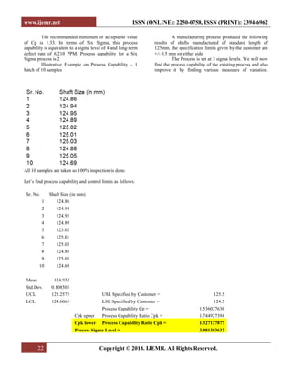
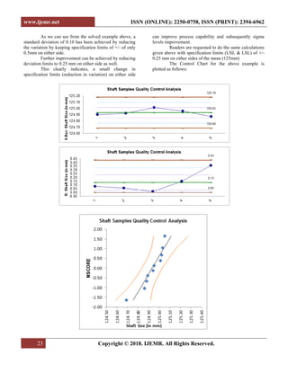
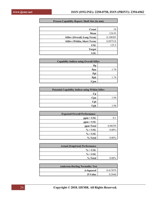
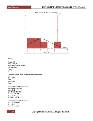
In this case paper the Process Capability achieved
was 1.74 and has been further improved to 1.94 resulting
in sigma level improvements from 5.22 to 5.82.
REFERENCES
[1] Bitran, G. R. & D. Tirupati. (1998). Planning and
scheduling for epitaxial wafer production facilities.
Operations Research, 36(1). 34-49.
[2] Bitran, G.R., E.A Haas, & A.C. Hax. (1981).
Hierarchical production planning: A single stage system.
Operations Research, 29, 717-743.
[3] Blackburn, J. & R. Millen. (1982). Improved heuristics
for multi-stage requirements planning. Management
Science, 28(1), 44-46.

Process Capability Analysis in Single and Multiple Batch Manufacturing Systems

More Related Content

What's hot

Similar to Process Capability Analysis in Single and Multiple Batch Manufacturing Systems

More from Dr. Amarjeet Singh

Recently uploaded

Process Capability Analysis in Single and Multiple Batch Manufacturing Systems