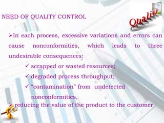
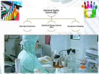
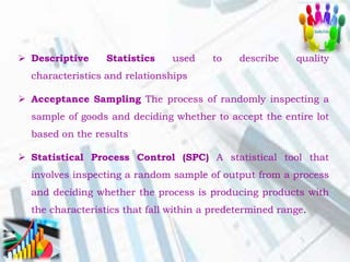
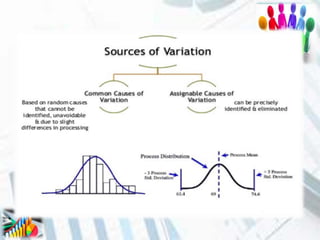
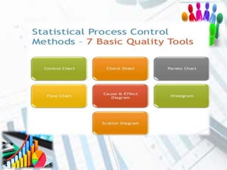
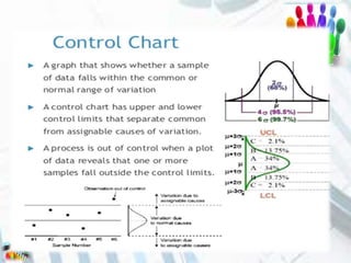
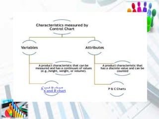
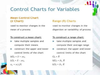
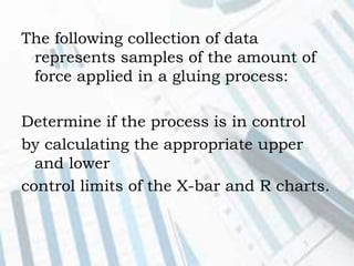
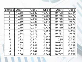
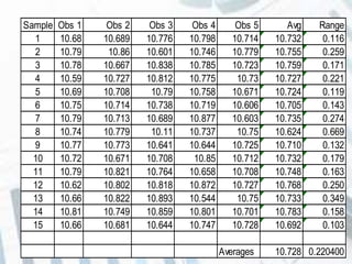
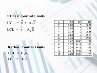
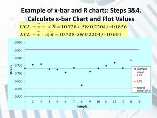
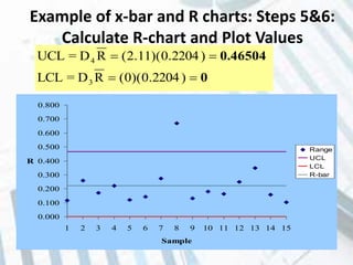
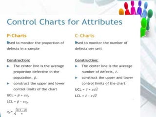
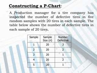
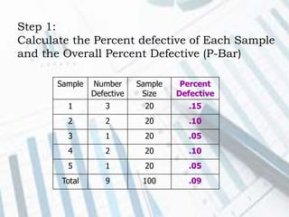
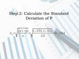
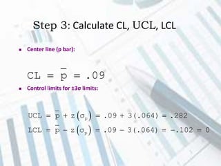
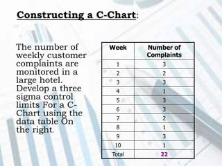
The word "Quality" represents the
properties of products and/or
services that are valued by the
consumer.
A system of maintaining standards
in manufactured products by
testing a sample of the output
against the specification.
In each process, excessive variations and errors can
cause nonconformities, which leads to three
undesirable consequences:
 scrapped or wasted resources;
 degraded process throughput;
 “contamination” from undetected
nonconformities,
 reducing the value of the product to the customer
NEED OF QUALITY CONTROL
GOAL OF QUALITY CONTROL
The goal of quality control in every production
system is to
 eliminate nonconformities and their consequences,
 eliminate rework and wasted resources, and
 achieve these goals at the lowest possible cost
A branch of mathematics used to
summarize, analyze, and
interpret a group of numbers or
observations.
Statistical quality control (SQC) is
the term used to describe the
set of statistical tools used by
quality professionals.
 Descriptive Statistics used to describe quality
characteristics and relationships
 Acceptance Sampling The process of randomly inspecting a
sample of goods and deciding whether to accept the entire lot
based on the results
 Statistical Process Control (SPC) A statistical tool that
involves inspecting a random sample of output from a process
and deciding whether the process is producing products with
the characteristics that fall within a predetermined range.
Why SPC is the Most Important Tool of
the SQC?
Measure the value of a quality characteristic
Help to identify a change or variation in some
quality characteristic of the product or process
Some Information about SPC
 SPC can be applied to any process.
 There is inherent variation in any process which can be
measured and “controlled”.
 SPC doesn’t eliminate variation, but it does allow the user to
track special cause variation.
 “SPC is a statistical method of separating variation resulting
from special causes from natural variation and to establish
and maintain consistency in the process, enabling process
improvement.”
x̅ and R chart
x̅ and R chart
x̅ and R chart
The following collection of data
represents samples of the amount of
force applied in a gluing process:
Determine if the process is in control
by calculating the appropriate upper
and lower
control limits of the X-bar and R charts.
Sample Obs 1 Obs 2 Obs 3 Obs 4 Obs 5
1 10.68 10.689 10.776 10.798 10.714
2 10.79 10.86 10.601 10.746 10.779
3 10.78 10.667 10.838 10.785 10.723
4 10.59 10.727 10.812 10.775 10.73
5 10.69 10.708 10.79 10.758 10.671
6 10.75 10.714 10.738 10.719 10.606
7 10.79 10.713 10.689 10.877 10.603
8 10.74 10.779 10.11 10.737 10.75
9 10.77 10.773 10.641 10.644 10.725
10 10.72 10.671 10.708 10.85 10.712
11 10.79 10.821 10.764 10.658 10.708
12 10.62 10.802 10.818 10.872 10.727
13 10.66 10.822 10.893 10.544 10.75
14 10.81 10.749 10.859 10.801 10.701
15 10.66 10.681 10.644 10.747 10.728
Sample Obs 1 Obs 2 Obs 3 Obs 4 Obs 5 Avg Range
1 10.68 10.689 10.776 10.798 10.714 10.732 0.116
2 10.79 10.86 10.601 10.746 10.779 10.755 0.259
3 10.78 10.667 10.838 10.785 10.723 10.759 0.171
4 10.59 10.727 10.812 10.775 10.73 10.727 0.221
5 10.69 10.708 10.79 10.758 10.671 10.724 0.119
6 10.75 10.714 10.738 10.719 10.606 10.705 0.143
7 10.79 10.713 10.689 10.877 10.603 10.735 0.274
8 10.74 10.779 10.11 10.737 10.75 10.624 0.669
9 10.77 10.773 10.641 10.644 10.725 10.710 0.132
10 10.72 10.671 10.708 10.85 10.712 10.732 0.179
11 10.79 10.821 10.764 10.658 10.708 10.748 0.163
12 10.62 10.802 10.818 10.872 10.727 10.768 0.250
13 10.66 10.822 10.893 10.544 10.75 10.733 0.349
14 10.81 10.749 10.859 10.801 10.701 10.783 0.158
15 10.66 10.681 10.644 10.747 10.728 10.692 0.103
Averages 10.728 0.220400
x Chart Control Limits
UCL = x + A R
LCL = x - A R
2
2
R Chart Control Limits
UCL = D R
LCL = D R
4
3
n A2 D3 D4
2 1.88 0 3.27
3 1.02 0 2.57
4 0.73 0 2.28
5 0.58 0 2.11
6 0.48 0 2.00
7 0.42 0.08 1.92
8 0.37 0.14 1.86
9 0.34 0.18 1.82
10 0.31 0.22 1.78
11 0.29 0.26 1.74
Example of x-bar and R charts: Steps 3&4.
Calculate x-bar Chart and Plot Values
60110220405872810
85610220405872810
2
2
.)=.(-..R- AxLCL =
.)=.(..R+ AxUCL =


10.550
10.600
10.650
10.700
10.750
10.800
10.850
10.900
1 2 3 4 5 6 7 8 9 10 11 12 13 14 15
Sample
Means
Sample
mean
UCL
LCL
grand
mean of x
Example of x-bar and R charts: Steps 5&6:
Calculate R-chart and Plot Values
0
0.46504


)2204.0)(0(RD=LCL
)2204.0)(11.2(RD=UCL
3
4
0.000
0.100
0.200
0.300
0.400
0.500
0.600
0.700
0.800
1 2 3 4 5 6 7 8 9 10 11 12 13 14 15
Sample
R
Range
UCL
LCL
R-bar
P chart & c-chart
Constructing a P-Chart:
A Production manager for a tire company has
inspected the number of defective tires in five
random samples with 20 tires in each sample. The
table below shows the number of defective tires in
each sample of 20 tires.
Sample Sample
Size (n)
Number
Defective
1 20 3
2 20 2
3 20 1
4 20 2
5 20 1
Step 1:
Calculate the Percent defective of Each Sample
and the Overall Percent Defective (P-Bar)
Sample Number
Defective
Sample
Size
Percent
Defective
1 3 20 .15
2 2 20 .10
3 1 20 .05
4 2 20 .10
5 1 20 .05
Total 9 100 .09
Step 2: Calculate the Standard
Deviation of P
p
p(1-p) (.09)(.91)
σ = = =0.064
n 20
Step 3: Calculate CL, UCL, LCL
CL p .09 
 Center line (p bar):
 Control limits for ±3σ limits:
 
 
p
p
UCL p z σ .09 3(.064) .282
LCL p z σ .09 3(.064) .102 0
    
      
Step 4: Draw the Chart
Constructing a C-Chart:
The number of
weekly customer
complaints are
monitored in a
large hotel.
Develop a three
sigma control
limits For a C-
Chart using the
data table On
the right.
Week Number of
Complaints
1 3
2 2
3 3
4 1
5 3
6 3
7 2
8 1
9 3
10 1
Total 22
Calculate CL, UCL, LCL
 Center line (c bar):
 Control limits for ±3σ limits:
UCL c c 2.2 3 2.2 6.65
LCL c c 2.2 3 2.2 2.25 0
z
z
    
      
#complaints 22
CL 2.2
# of samples 10
  
Step 4: Draw the Chart
Statistical quality control

Statistical quality control

  • 2.
    The word "Quality"represents the properties of products and/or services that are valued by the consumer.
  • 3.
    A system ofmaintaining standards in manufactured products by testing a sample of the output against the specification.
  • 4.
    In each process,excessive variations and errors can cause nonconformities, which leads to three undesirable consequences:  scrapped or wasted resources;  degraded process throughput;  “contamination” from undetected nonconformities,  reducing the value of the product to the customer NEED OF QUALITY CONTROL
  • 5.
    GOAL OF QUALITYCONTROL The goal of quality control in every production system is to  eliminate nonconformities and their consequences,  eliminate rework and wasted resources, and  achieve these goals at the lowest possible cost
  • 7.
    A branch ofmathematics used to summarize, analyze, and interpret a group of numbers or observations.
  • 8.
    Statistical quality control(SQC) is the term used to describe the set of statistical tools used by quality professionals.
  • 10.
     Descriptive Statisticsused to describe quality characteristics and relationships  Acceptance Sampling The process of randomly inspecting a sample of goods and deciding whether to accept the entire lot based on the results  Statistical Process Control (SPC) A statistical tool that involves inspecting a random sample of output from a process and deciding whether the process is producing products with the characteristics that fall within a predetermined range.
  • 11.
    Why SPC isthe Most Important Tool of the SQC? Measure the value of a quality characteristic Help to identify a change or variation in some quality characteristic of the product or process
  • 12.
    Some Information aboutSPC  SPC can be applied to any process.  There is inherent variation in any process which can be measured and “controlled”.  SPC doesn’t eliminate variation, but it does allow the user to track special cause variation.  “SPC is a statistical method of separating variation resulting from special causes from natural variation and to establish and maintain consistency in the process, enabling process improvement.”
  • 17.
    x̅ and Rchart x̅ and R chart
  • 18.
    x̅ and Rchart
  • 20.
    The following collectionof data represents samples of the amount of force applied in a gluing process: Determine if the process is in control by calculating the appropriate upper and lower control limits of the X-bar and R charts.
  • 21.
    Sample Obs 1Obs 2 Obs 3 Obs 4 Obs 5 1 10.68 10.689 10.776 10.798 10.714 2 10.79 10.86 10.601 10.746 10.779 3 10.78 10.667 10.838 10.785 10.723 4 10.59 10.727 10.812 10.775 10.73 5 10.69 10.708 10.79 10.758 10.671 6 10.75 10.714 10.738 10.719 10.606 7 10.79 10.713 10.689 10.877 10.603 8 10.74 10.779 10.11 10.737 10.75 9 10.77 10.773 10.641 10.644 10.725 10 10.72 10.671 10.708 10.85 10.712 11 10.79 10.821 10.764 10.658 10.708 12 10.62 10.802 10.818 10.872 10.727 13 10.66 10.822 10.893 10.544 10.75 14 10.81 10.749 10.859 10.801 10.701 15 10.66 10.681 10.644 10.747 10.728
  • 22.
    Sample Obs 1Obs 2 Obs 3 Obs 4 Obs 5 Avg Range 1 10.68 10.689 10.776 10.798 10.714 10.732 0.116 2 10.79 10.86 10.601 10.746 10.779 10.755 0.259 3 10.78 10.667 10.838 10.785 10.723 10.759 0.171 4 10.59 10.727 10.812 10.775 10.73 10.727 0.221 5 10.69 10.708 10.79 10.758 10.671 10.724 0.119 6 10.75 10.714 10.738 10.719 10.606 10.705 0.143 7 10.79 10.713 10.689 10.877 10.603 10.735 0.274 8 10.74 10.779 10.11 10.737 10.75 10.624 0.669 9 10.77 10.773 10.641 10.644 10.725 10.710 0.132 10 10.72 10.671 10.708 10.85 10.712 10.732 0.179 11 10.79 10.821 10.764 10.658 10.708 10.748 0.163 12 10.62 10.802 10.818 10.872 10.727 10.768 0.250 13 10.66 10.822 10.893 10.544 10.75 10.733 0.349 14 10.81 10.749 10.859 10.801 10.701 10.783 0.158 15 10.66 10.681 10.644 10.747 10.728 10.692 0.103 Averages 10.728 0.220400
  • 23.
    x Chart ControlLimits UCL = x + A R LCL = x - A R 2 2 R Chart Control Limits UCL = D R LCL = D R 4 3 n A2 D3 D4 2 1.88 0 3.27 3 1.02 0 2.57 4 0.73 0 2.28 5 0.58 0 2.11 6 0.48 0 2.00 7 0.42 0.08 1.92 8 0.37 0.14 1.86 9 0.34 0.18 1.82 10 0.31 0.22 1.78 11 0.29 0.26 1.74
  • 24.
    Example of x-barand R charts: Steps 3&4. Calculate x-bar Chart and Plot Values 60110220405872810 85610220405872810 2 2 .)=.(-..R- AxLCL = .)=.(..R+ AxUCL =   10.550 10.600 10.650 10.700 10.750 10.800 10.850 10.900 1 2 3 4 5 6 7 8 9 10 11 12 13 14 15 Sample Means Sample mean UCL LCL grand mean of x
  • 25.
    Example of x-barand R charts: Steps 5&6: Calculate R-chart and Plot Values 0 0.46504   )2204.0)(0(RD=LCL )2204.0)(11.2(RD=UCL 3 4 0.000 0.100 0.200 0.300 0.400 0.500 0.600 0.700 0.800 1 2 3 4 5 6 7 8 9 10 11 12 13 14 15 Sample R Range UCL LCL R-bar
  • 26.
    P chart &c-chart
  • 28.
    Constructing a P-Chart: AProduction manager for a tire company has inspected the number of defective tires in five random samples with 20 tires in each sample. The table below shows the number of defective tires in each sample of 20 tires. Sample Sample Size (n) Number Defective 1 20 3 2 20 2 3 20 1 4 20 2 5 20 1
  • 29.
    Step 1: Calculate thePercent defective of Each Sample and the Overall Percent Defective (P-Bar) Sample Number Defective Sample Size Percent Defective 1 3 20 .15 2 2 20 .10 3 1 20 .05 4 2 20 .10 5 1 20 .05 Total 9 100 .09
  • 30.
    Step 2: Calculatethe Standard Deviation of P p p(1-p) (.09)(.91) σ = = =0.064 n 20
  • 31.
    Step 3: CalculateCL, UCL, LCL CL p .09   Center line (p bar):  Control limits for ±3σ limits:     p p UCL p z σ .09 3(.064) .282 LCL p z σ .09 3(.064) .102 0            
  • 32.
    Step 4: Drawthe Chart
  • 33.
    Constructing a C-Chart: Thenumber of weekly customer complaints are monitored in a large hotel. Develop a three sigma control limits For a C- Chart using the data table On the right. Week Number of Complaints 1 3 2 2 3 3 4 1 5 3 6 3 7 2 8 1 9 3 10 1 Total 22
  • 34.
    Calculate CL, UCL,LCL  Center line (c bar):  Control limits for ±3σ limits: UCL c c 2.2 3 2.2 6.65 LCL c c 2.2 3 2.2 2.25 0 z z             #complaints 22 CL 2.2 # of samples 10   
  • 35.
    Step 4: Drawthe Chart