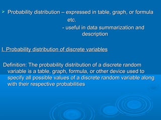
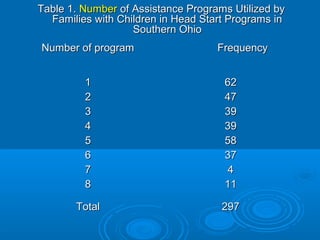
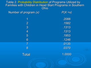
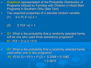
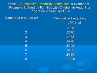
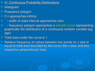
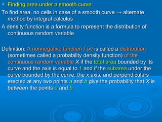
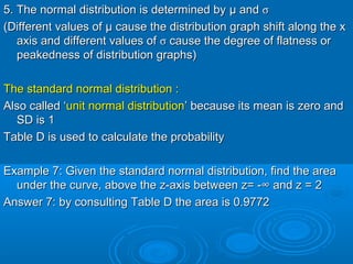
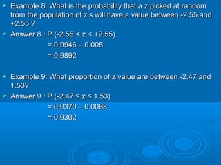
This document discusses probability distributions and provides examples of calculating probabilities using binomial distributions. It begins by defining a probability distribution as a table, graph or formula used to specify the possible values and probabilities of a discrete random variable. It then gives examples of probability distributions for number of assistance programs used by families and calculates related probabilities. The document introduces binomial distribution and provides two examples of calculating probabilities of outcomes for binomial processes, such as number of full term births out of total births. It describes key concepts like Bernoulli trials, processes and use of combinations and factorials to calculate probabilities for larger sample sizes.

1. PROBABILITY DISTRIBUTIONPROBABILITY DISTRIBUTION
Dr Htin Zaw SoeDr Htin Zaw Soe
MBBS, DFT, MMedSc (P & TM), PhD, DipMedEdMBBS, DFT, MMedSc (P & TM), PhD, DipMedEd
Associate ProfessorAssociate Professor
Department of BiostatisticsDepartment of Biostatistics
University of Public HealthUniversity of Public Health

2.  Probability distribution – expressed in table, graph, or formulaProbability distribution – expressed in table, graph, or formula
etc.etc.
- useful in data summarization and- useful in data summarization and
descriptiondescription
I. Probability distribution of discrete variablesI. Probability distribution of discrete variables
Definition: The probability distribution of a discrete randomDefinition: The probability distribution of a discrete random
variable is a table, graph, formula, or other device used tovariable is a table, graph, formula, or other device used to
specify all possible values of a discrete random variable alongspecify all possible values of a discrete random variable along
with their respective probabilitieswith their respective probabilities

3. Table 1.Table 1. NumberNumber of Assistance Programs Utilized byof Assistance Programs Utilized by
Families with Children in Head Start Programs inFamilies with Children in Head Start Programs in
Southern OhioSouthern Ohio
Number of programNumber of program FrequencyFrequency
11
22
33
44
55
66
77
88
6262
4747
3939
3939
5858
3737
44
1111
TotalTotal 297297

4. Table 2.Table 2. Probability DistributionProbability Distribution of Programs Utilized byof Programs Utilized by
Families with Children in Head Start Programs in SouthernFamilies with Children in Head Start Programs in Southern
OhioOhio
Number of programNumber of program (x)(x) P(X =x)P(X =x)
11
22
33
44
55
66
77
88
.2088.2088
.1582.1582
.1313.1313
.1313.1313
.1953.1953
.1246.1246
.0135.0135
.0370.0370
TotalTotal 1.00001.0000

5.  GraphicalGraphical representation of the Probability Distribution ofrepresentation of the Probability Distribution of
Programs Utilized by Families with Children in Head StartPrograms Utilized by Families with Children in Head Start
Programs in Southern Ohio (See Text)Programs in Southern Ohio (See Text)
 Two essential properties of a discrete random variableTwo essential properties of a discrete random variable
(1) 0(1) 0 ≤≤ P( X =x)P( X =x) ≤≤ 11
(2)(2) ΣΣ P(X =x)P(X =x) = 1= 1
 Q1Q1: What is the probability that a randomly selected family: What is the probability that a randomly selected family
will be one who used three assistance programs?will be one who used three assistance programs?
A1A1:: P(X =P(X = 3) is 0.13133) is 0.1313
 Q1Q1: What is the probability that a randomly selected family: What is the probability that a randomly selected family
used either oneused either one oror two programs?two programs?
A1A1:: PP(1(1UU 2) =2) = PP(1) +(1) + PP (2) = 0.2088 + 0.1582(2) = 0.2088 + 0.1582
= 0.3670= 0.3670

6. Table 3.Table 3. CumulativeCumulative Probability DistributionProbability Distribution of Number ofof Number of
Programs Utilized by Families with Children in Head StartPrograms Utilized by Families with Children in Head Start
Programs in Southern OhioPrograms in Southern Ohio
Number of programNumber of program (x)(x) CumulativeCumulative FrequencyFrequency
(PX(PX ≤≤ x)x)
11
22
33
44
55
66
77
88
.2088.2088
.3670.3670
.4983.4983
.6296.6296
.8249.8249
.9495.9495
.9630.9630
1.00001.0000

7.  Cumulative Probability forCumulative Probability for xxii is written asis written as F (xF (xii)) == P(XP(X ≤ x≤ xii))
[[ XX is less than or equal to a specified value,is less than or equal to a specified value, xxii
eg.eg. FF (2) =(2) = PP (( XX ≤ 2) ]≤ 2) ]
The graph of a cumulativeThe graph of a cumulative probability distribution is called ‘probability distribution is called ‘OgiveOgive’’..
(See text)(See text)
By consulting the cumulativeBy consulting the cumulative probability distribution we canprobability distribution we can
answer the following questionsanswer the following questions
Q 3Q 3: What is the probability that a family picked at random will be: What is the probability that a family picked at random will be
one who used twoone who used two oror fewer programs?fewer programs?
Q 4Q 4: What is the probability that a family picked at random will be: What is the probability that a family picked at random will be
one who used fewer than four programs?one who used fewer than four programs?
Q 5Q 5: What is the probability that a family picked at random will be: What is the probability that a family picked at random will be
one who used fiveone who used five oror more programs?more programs?
Q 6Q 6: What is the probability that a family picked at random will be: What is the probability that a family picked at random will be
one who used between three and five programs, inclusive?one who used between three and five programs, inclusive?

8.  A3: P (XA3: P (X ≤ 2) = 0.3670≤ 2) = 0.3670
 A4: P ( X < 4A4: P ( X < 4) = P (X ≤ 3) = 0.4983) = P (X ≤ 3) = 0.4983
 A5: P (X ≥ 5) = 1 – 0.6296 = 0.3704A5: P (X ≥ 5) = 1 – 0.6296 = 0.3704
 A6: P ( 3 ≤ X ≤ 5) = 0.8249 – 0.3670 = 0.4579A6: P ( 3 ≤ X ≤ 5) = 0.8249 – 0.3670 = 0.4579

9.  Three basic probability distributionsThree basic probability distributions
(1) The binomial distribution(1) The binomial distribution
(2) The Poisson distribution(2) The Poisson distribution
(3) The normal distribution(3) The normal distribution

10. II. The binomial distributionII. The binomial distribution
- Derived from a- Derived from a BernoulliBernoulli trial or process [Swiss Mathematiciantrial or process [Swiss Mathematician
James Bernoulli (1654-1705)]James Bernoulli (1654-1705)]
- When a random process or experiment or a trial can result in- When a random process or experiment or a trial can result in
only one of two mutually exclusive outcomes such as dead oronly one of two mutually exclusive outcomes such as dead or
alive, sick or well, full-term or premature, the trial is known as aalive, sick or well, full-term or premature, the trial is known as a
BernoulliBernoulli trial.trial.

11.  TheThe BernoulliBernoulli processprocess
TheThe BernoulliBernoulli trials forms atrials forms a BernoulliBernoulli processprocess under theunder the
following conditions.following conditions.
(1) Each trial results in(1) Each trial results in one of two mutually exclusive outcomesone of two mutually exclusive outcomes..
One the success, the other failureOne the success, the other failure
(2) The probability of a(2) The probability of a success (success (pp)) remains constant from trial toremains constant from trial to
trial. The probability oftrial. The probability of failure (failure (1- p1- p) is denoted by () is denoted by (qq))
(3) The trials are(3) The trials are independentindependent; that is the outcome of any; that is the outcome of any
particular trial is not affected by the outcome of any other trial.particular trial is not affected by the outcome of any other trial.

12.  Example 1: 85.8 % of pregnancies had full-term birth. What isExample 1: 85.8 % of pregnancies had full-term birth. What is
the probability thatthe probability that exactly three of fiveexactly three of five birth records randomlybirth records randomly
selected from that population will be full-term birth?selected from that population will be full-term birth?
FPFFP (F= Full-term, P=Premature)FPFFP (F= Full-term, P=Premature)
10110 (Coded form: F=1, P=0)10110 (Coded form: F=1, P=0)
According toAccording to multiplication rulemultiplication rule probability of above sequence is:probability of above sequence is:
P(1, 0, 1, 1, 0) =P(1, 0, 1, 1, 0) = pqppq = qpqppq = q22
pp33
NumberNumber SequenceSequence NumberNumber SequenceSequence
2 11100 7 011102 11100 7 01110
3 10011 8 001113 10011 8 00111
4 11010 9 010114 11010 9 01011
5 11001 10 011015 11001 10 01101
6 101016 10101

13.  According toAccording to addition ruleaddition rule,,
the probability is sum of individual probabilitiesthe probability is sum of individual probabilities
ie. 10ie. 10 × q× q22
pp33
pp = 0.858,= 0.858, qq = 1 - 0.858 = 0.142= 1 - 0.858 = 0.142
10 × (0.142)10 × (0.142)22
(0.858)(0.858) 33
= 0.1276= 0.1276

14.  Large sample procedure: Use of ‘combination’Large sample procedure: Use of ‘combination’
 If a set consists ofIf a set consists of nn objects, and we wish to form a subset ofobjects, and we wish to form a subset of xx
objects from theseobjects from these nn objects, without regard to the order of theobjects, without regard to the order of the
objects in the subset, the result is called aobjects in the subset, the result is called a combinationcombination
 Definition of combination: ADefinition of combination: A combinationcombination ofof nn objects takenobjects taken xx atat
a time is an unordered subset ofa time is an unordered subset of xx ofof nn objectsobjects
nn CC xx == nn ! /! / xx ! (! ( nn –– xx) ! ( ! is read factorial)) ! ( ! is read factorial)
55 CC 33 = 5= 5 ! / 3 ! ( 5 – 3) !! / 3 ! ( 5 – 3) !
= 5 · 4 ·3 · 2 · 1 / 3 · 2 · 1 · 2 · 1= 5 · 4 ·3 · 2 · 1 / 3 · 2 · 1 · 2 · 1
= 120 / 12= 120 / 12
= 10= 10
[Note 1: 0[Note 1: 0 ! = 1]! = 1]

15.  Example 2: Smoking prevalence is 14% among pregnantExample 2: Smoking prevalence is 14% among pregnant
women in a county . If a random sample of size 10 selectedwomen in a county . If a random sample of size 10 selected
from that population, what is the probability that it will containsfrom that population, what is the probability that it will contains
exactly 4 mothers smoke during pregnancy?exactly 4 mothers smoke during pregnancy?
 f (x) =f (x) = nn CC xx qq n-xn-x
pp xx
nn CC xx == nn ! /! / xx ! (! ( nn –– xx) !) !
1010 CC 44 = 10= 10 ! / 4 ! ( 10 – 4) !! / 4 ! ( 10 – 4) !
== 1010 ! / 4 ! 6 !! / 4 ! 6 !
= 210= 210
f (x) =f (x) = nn CC xx qq n-xn-x
pp xx
f (4) = 210f (4) = 210 (.86)(.86) 10-410-4
(.14)(.14) 44
= 210= 210 (.86)(.86)66
(.14)(.14) 44

16.  Using Binomial Table (Table B)Using Binomial Table (Table B)
 Example 3: Smoking prevalence is 14% among pregnantExample 3: Smoking prevalence is 14% among pregnant
women in a county . If a random sample of size 10 selectedwomen in a county . If a random sample of size 10 selected
from that population, what is the probability that it will containsfrom that population, what is the probability that it will contains
exactly 4exactly 4 mothers smoke during pregnancy?mothers smoke during pregnancy?
n = 10, p = .14, x = 4n = 10, p = .14, x = 4
 Table B. Cumulative binomial probability distributionTable B. Cumulative binomial probability distribution
f (4) = P ( Xf (4) = P ( X≤ 4) -≤ 4) - P ( XP ( X≤ 3)≤ 3)
= .9927 - .9600= .9927 - .9600
= .0327= .0327

17.  Using Binomial Table (Table B) when p > 0.5Using Binomial Table (Table B) when p > 0.5
 Table B does not contain value ofTable B does not contain value of pp > 0.5. So> 0.5. So
P ( X = xP ( X = x || n , p > .5n , p > .5) =) = P ( X = n – xP ( X = n – x | n| n , 1- p, 1- p))
P ( XP ( X ≤≤ xx || n , p > .5n , p > .5) =) = P ( XP ( X ≥≥ n – xn – x | n| n , 1- p, 1- p))
When X is greater than or equal to some x whenWhen X is greater than or equal to some x when p > .5, usep > .5, use
P ( XP ( X ≥≥ xx || n , p > .5n , p > .5) =) = P ( XP ( X ≤≤ n – xn – x | n| n , 1- p, 1- p))

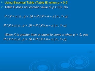
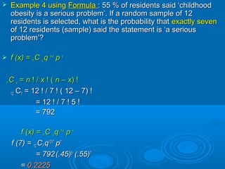
18.  Example 4 usingExample 4 using Table BTable B: 55 % of residents said ‘childhood: 55 % of residents said ‘childhood
obesity is a serious problem’. If a random sample of 12obesity is a serious problem’. If a random sample of 12
residents is selected, what is the probability thatresidents is selected, what is the probability that exactly sevenexactly seven
of 12 residents (sample) said the statement is ‘a seriousof 12 residents (sample) said the statement is ‘a serious
problem’?problem’?
P ( X = xP ( X = x || n , p > .5n , p > .5) =) = P ( X = n – xP ( X = n – x | n| n , 1- p, 1- p))
P ( X = 7P ( X = 7 || 12 , p > .5512 , p > .55) =) = P ( X = 5P ( X = 5 | 12| 12 , p =.45, p =.45))
P ( X = 5P ( X = 5 | 12| 12 , p =.45, p =.45) = P (X ≤ 5) - P (X ≤ 4)) = P (X ≤ 5) - P (X ≤ 4)
= .5269 - .3044= .5269 - .3044 ←← [From Table B][From Table B]
== .2225.2225

19.  Example 4 usingExample 4 using FormulaFormula : 55 % of residents said ‘childhood: 55 % of residents said ‘childhood
obesity is a serious problem’. If a random sample of 12obesity is a serious problem’. If a random sample of 12
residents is selected, what is the probability thatresidents is selected, what is the probability that exactly sevenexactly seven
of 12 residents (sample) said the statement is ‘a seriousof 12 residents (sample) said the statement is ‘a serious
problem’?problem’?
 f (x) =f (x) = nn CC xx qq n-xn-x
pp xx
nn CC xx == nn ! /! / xx ! (! ( nn –– xx) !) !
1212 CC77 = 12= 12 ! / 7 ! ( 12 – 7) !! / 7 ! ( 12 – 7) !
== 1212 ! / 7 ! 5 !! / 7 ! 5 !
= 792= 792
f (x) =f (x) = nn CC xx qq n-xn-x
pp xx
f (7) =f (7) = 1212 CC77 qq12-712-7
pp77
= 792= 792(.45)(.45)55
(.55)(.55)77
== 0.22250.2225

20. [Note 2: How to calculate 12[Note 2: How to calculate 12 !! // 7 ! 5 ! by an easier method ?7 ! 5 ! by an easier method ?
1212 !! // 7 ! 5 ! = 12·11·10·9·8·7·6·5·4·3·2·17 ! 5 ! = 12·11·10·9·8·7·6·5·4·3·2·1// (7·6·5·4·2·3·2·1) 5·4·3·2·1(7·6·5·4·2·3·2·1) 5·4·3·2·1
= 12·11·10·9·8= 12·11·10·9·8 7 !7 ! // 7 !7 ! 5·4·3·2·15·4·3·2·1
= 12·11·10·9·8= 12·11·10·9·8 // 5·4·3·2·15·4·3·2·1
= 792 ]= 792 ]
[Note 3: mean of binomial distribution =[Note 3: mean of binomial distribution = μμ == npnp
variancevariance of binomial distribution =of binomial distribution = σσ 22
== np (1-p)np (1-p) ]]

21.  III. The Poisson DistributionIII. The Poisson Distribution
[French Mathematician Denis Poisson (1781 – 1840)][French Mathematician Denis Poisson (1781 – 1840)]
 IfIf xx is the number of occurrences of some random event in anis the number of occurrences of some random event in an
interval of time or space (or some volume of matter), theinterval of time or space (or some volume of matter), the
probability thatprobability that xx will occur is given by:will occur is given by:
 f (x) = ef (x) = e--λλ
λλ xx
/ x/ x !!
 (( λλ = a parameter of the distribution, the average number of= a parameter of the distribution, the average number of
occurrences of the random event in the interval or volume;occurrences of the random event in the interval or volume;
e = a constant , 2.7183)e = a constant , 2.7183)

22.  The Poisson ProcessThe Poisson Process states that:states that:
1. The occurrences of the events are1. The occurrences of the events are independentindependent. The. The
occurrence of an event in an interval of space or time has nooccurrence of an event in an interval of space or time has no
effect on the probability of a second occurrence of the event ineffect on the probability of a second occurrence of the event in
the same, or any other, intervalthe same, or any other, interval
2. Theoretically2. Theoretically an infinite numberan infinite number of occurrences of the eventof occurrences of the event
must be possible in the intervalmust be possible in the interval
3. The probability of the3. The probability of the single occurrencesingle occurrence of the event in a givenof the event in a given
interval isinterval is proportional to the length of the intervalproportional to the length of the interval
4. In an4. In an infinitesimally smallinfinitesimally small portion of the interval, the probabilityportion of the interval, the probability
of more than one occurrence of the event isof more than one occurrence of the event is negligiblenegligible
Mean and variance are equal in Poisson distributionMean and variance are equal in Poisson distribution

23.  When to use the Poisson Model?When to use the Poisson Model?
 When counts are made of events or entities that are distributedWhen counts are made of events or entities that are distributed
at random in space or time the Poisson Model is usedat random in space or time the Poisson Model is used
 Example 5: Accidental poisoning cases admitted to a generalExample 5: Accidental poisoning cases admitted to a general
hospital follow the Poisson Law withhospital follow the Poisson Law with λλ = 12 cases per year.= 12 cases per year.
Find probability that in the next yearFind probability that in the next year exactly threeexactly three cases will becases will be
admitted to the hospital.admitted to the hospital.
f (x) = ef (x) = e--λλ
λλ xx
/ x/ x !!
P (X =3) = eP (X =3) = e--λλ
λλ xx
/ x/ x !!
== 2.71832.7183 ––1212
1212 33
/ 3/ 3 !!
= .00177= .00177

24.  Example 6: Average number of certain aquatic organism in aExample 6: Average number of certain aquatic organism in a
water sample taken from a pond is found to be 2. If the numberwater sample taken from a pond is found to be 2. If the number
follow the Poisson Law, find the probability that next sample willfollow the Poisson Law, find the probability that next sample will
containcontain one or fewerone or fewer organism.organism.
P (XP (X ≤ 1≤ 1) = P (X) = P (X =0=0) + P (X =) + P (X = 11))
= e= e--λλ
λλ xx
/ x/ x ! +! + ee--λλ
λλ xx
/ x/ x !!
== 2.71832.7183 ––22
22 00
/ 0/ 0 ! +! + 2.71832.7183 ––22
22 11
/ 1/ 1 !!
= .1353 + .27067= .1353 + .27067
= .406= .406
We can get answer easily by consulting Table CWe can get answer easily by consulting Table C
P (XP (X ≤ 1≤ 1) =) = .406.406

25.  IV. Continuous Probability DistributionsIV. Continuous Probability Distributions
 HistogramHistogram
 Frequency polygonFrequency polygon
 IfIf nn approaches infinity,approaches infinity,
 - width of class interval approaches zero.- width of class interval approaches zero.
 - frequency polygon approaches a- frequency polygon approaches a smooth curvesmooth curve representingrepresenting
graphically the distribution of a continuous random variable (eg.graphically the distribution of a continuous random variable (eg.
age)age)
 Total area under the curve is 1Total area under the curve is 1
 Relative frequency of values between two points onRelative frequency of values between two points on xx axis isaxis is
equal to total area bounded by the curve, theequal to total area bounded by the curve, the xx axis, and twoaxis, and two
respective perpendicular lines.respective perpendicular lines.

26.  Finding area under a smooth curve:Finding area under a smooth curve:
To find area, no cells in case of a smooth curveTo find area, no cells in case of a smooth curve →→ alternatealternate
methodmethod by integral calculusby integral calculus
A density function is a formula to represent the distribution ofA density function is a formula to represent the distribution of
continuous random variablecontinuous random variable
Definition:Definition: A nonnegative functionA nonnegative function f (x)f (x) is called ais called a distributiondistribution
(sometimes called a probability density function)(sometimes called a probability density function) of theof the
continuous random variablecontinuous random variable XX if theif the total areatotal area bounded by itsbounded by its
curve and the axis is equal tocurve and the axis is equal to 11 and if theand if the subareasubarea under theunder the
curve bounded by the curve, thecurve bounded by the curve, the xx axis, and perpendicularsaxis, and perpendiculars
erected at any two pointserected at any two points aa andand bb give the probability thatgive the probability that XX isis
between the pointsbetween the points aa andand bb..

27.  IV. The Normal DistributionIV. The Normal Distribution
The Gaussian distribution [Carl Friedrich Gauss (1777-1855)]The Gaussian distribution [Carl Friedrich Gauss (1777-1855)]
The normal density is:The normal density is:
f (x) = (1/f (x) = (1/√√ 22ππσσ ) e) e-(x--(x- µµ)2/2)2/2σσ22
( -( -∞∞< x << x < ∞)∞)
 Characteristics of the normal distributionCharacteristics of the normal distribution
1. It is symmetrical about the mean,1. It is symmetrical about the mean, µ . The curve on either side ofµ . The curve on either side of
µ is mirror image of the other sideµ is mirror image of the other side
2. The mean, the median and mode are all equal.2. The mean, the median and mode are all equal.
3. The total area under the curve above the x axis is3. The total area under the curve above the x axis is one squareone square
unitunit. Normal distribution is probability distribution. 50% of the. Normal distribution is probability distribution. 50% of the
area is to the right of a perpendicular erected at the mean andarea is to the right of a perpendicular erected at the mean and
50% is to the left.50% is to the left.
4. 1 SD from the mean in both directions, the area is 68%.4. 1 SD from the mean in both directions, the area is 68%.
For 2 SD and 3 SD, areas are 95% and 99.7% respectivelyFor 2 SD and 3 SD, areas are 95% and 99.7% respectively

28. 5. The normal distribution is determined by5. The normal distribution is determined by µ andµ and σσ
(Different values of(Different values of µµ cause the distribution graph shift along the xcause the distribution graph shift along the x
axis and different values ofaxis and different values of σσ cause the degree of flatness orcause the degree of flatness or
peakedness of distribution graphs)peakedness of distribution graphs)
The standard normal distribution :The standard normal distribution :
Also called ‘Also called ‘unit normal distributionunit normal distribution’ because its mean is zero and’ because its mean is zero and
SD is 1SD is 1
Table D is used to calculate the probabilityTable D is used to calculate the probability
Example 7: Given the standard normal distribution, find the areaExample 7: Given the standard normal distribution, find the area
under the curve, above the z-axis between z= -∞ and z = 2under the curve, above the z-axis between z= -∞ and z = 2
Answer 7: by consulting Table D the area is 0.9772Answer 7: by consulting Table D the area is 0.9772

29.  Example 8: What is the probability that a z picked at randomExample 8: What is the probability that a z picked at random
from the population of z’s will have a value between -2.55 andfrom the population of z’s will have a value between -2.55 and
+2.55 ?+2.55 ?
 Answer 8 : P (Answer 8 : P (-2.55 < z < +2.55)-2.55 < z < +2.55)
= 0.9946 – 0.005= 0.9946 – 0.005
= 0.9892= 0.9892
 Example 9: What proportion of z value are between -2.47 andExample 9: What proportion of z value are between -2.47 and
1.53?1.53?
 Answer 9 : P (Answer 9 : P (-2.47-2.47 ≤≤ zz ≤≤ 1.53)1.53)
= 0.9370 – 0.0068= 0.9370 – 0.0068
= 0.9302= 0.9302

30.  Example 10: Given the standard normal distribution,Example 10: Given the standard normal distribution,
findfind P (z ≥2.71)P (z ≥2.71)
 Answer 10 : P (z ≥2.71)Answer 10 : P (z ≥2.71)
= 1 –= 1 – P (z ≤ 2.71)P (z ≤ 2.71)
= 1 - 0.9966= 1 - 0.9966
= 0.0034= 0.0034

31.  Normal Distribution ApplicationsNormal Distribution Applications
- To makeTo make probabilityprobability statement by using normal distributionstatement by using normal distribution
- Example 11: Amount of time children (8-15 yr) spent in theExample 11: Amount of time children (8-15 yr) spent in the
upright position in 24 hr followed a normal distribution with aupright position in 24 hr followed a normal distribution with a
mean of 5.4 hr and SD of 1.3 hr. Find the prob. that a childmean of 5.4 hr and SD of 1.3 hr. Find the prob. that a child
selected at random spends less than 3 hr in upright position inselected at random spends less than 3 hr in upright position in
24 hr period.24 hr period.
- Answer 11:Answer 11:
z = x-z = x- µµ // σσ
= 3 – 5.4 / 1.3= 3 – 5.4 / 1.3
= - 1.85= - 1.85
By consulting Table DBy consulting Table D
P (x < 3) = P ( z < - 1.85) = 0.0322P (x < 3) = P ( z < - 1.85) = 0.0322

32. - Example 12: In a study of a common breath metabolite,Example 12: In a study of a common breath metabolite,
ammonia concentration (ppb) in a subject followed a normalammonia concentration (ppb) in a subject followed a normal
distribution over 30 days with a mean of 491ppb and SD 119distribution over 30 days with a mean of 491ppb and SD 119
ppb. What is the prob. that on a random day, the subject’sppb. What is the prob. that on a random day, the subject’s
ammonia conc. is between 292 and 649 ppb?ammonia conc. is between 292 and 649 ppb?
- Answer 12:Answer 12:
z = x-z = x- µµ // σσ
P ( 292 ≤ x ≤ 649 ) = P (P ( 292 ≤ x ≤ 649 ) = P ( x-x- µµ // σσ ≤ z ≤≤ z ≤ x-x- µµ // σσ))
= P (= P ( 292 - 491 / 119292 - 491 / 119 ≤ z ≤ 649≤ z ≤ 649 - 491 / 119- 491 / 119))
= P (= P ( - 1.67- 1.67 ≤ z ≤≤ z ≤ 1.331.33))
= 0.9082 – 0.0475= 0.9082 – 0.0475
= 0.8607= 0.8607

33.  Example 13: In a population of 10,000 of the children inExample 13: In a population of 10,000 of the children in
example 11, how many would you expect to be upright moreexample 11, how many would you expect to be upright more
than 8.5 hr? (mean, 5.4 hr and SD, 1.3 hr)than 8.5 hr? (mean, 5.4 hr and SD, 1.3 hr)
- Answer 13:Answer 13:
z = x-z = x- µµ // σσ
P ( x ≥ 8.5 ) = 1 - P ( x ≤ 8.5 )P ( x ≥ 8.5 ) = 1 - P ( x ≤ 8.5 )
= 1 - P ( z == 1 - P ( z = x-x- µµ // σσ ))
= 1 - P ( z =8.5= 1 - P ( z =8.5 – 5.4 / 1.3– 5.4 / 1.3 ))
= 1 - P ( z = 2.38 )= 1 - P ( z = 2.38 )
= 1 – 0. 9913= 1 – 0. 9913
= 0. 0087= 0. 0087
For population , we expect 10,000 (0.0087) = 87 children to spendFor population , we expect 10,000 (0.0087) = 87 children to spend
more than 8.5 hr upright.more than 8.5 hr upright.

34. THE ENDTHE END