This document is a thesis submitted by Omar Ghazi Abbood Khukre to the Department of Information Technology at Alexandria University in partial fulfillment of the requirements for a Master's degree in Information Technology. The thesis proposes a lossy image compression approach using Stationary Wavelet Transform and Vector Quantization. It includes acknowledgments, an abstract, table of contents, list of figures/tables, and chapters on introduction, background/literature review, the proposed lossy compression method, experiments and results analysis, and conclusion.

1. Lossy Compression Using Stationary Wavelet
Transform and Vector Quantization
Thesis Submitted to
Department of Information Technology
Institute of Graduate Studies and Research
Alexandria University
In Partial Fulfillment of the Requirements
For the Degree
Of
Master
In
Information Technology
By
Omar Ghazi Abbood Khukre
B.Sc. of Computer Science – 2011
Al-Turath University College, IRAQ-Baghdad
2016

2. Lossy Compression Using Stationary Wavelet
Transform and Vector Quantization
A Thesis
Presented by
Omar Ghazi Abbood Khukre
For the Degree of
Master
In
Information Technology
Examiners’ Committee: Approved
Prof. Dr. Mahmoud Mohamed Hassan Gabr
Prof. of Mathematics,
Faculty of science,
Alexandria University
…………………….
Prof. Dr. Abd El Baith Mohamed Mohamed
Prof. of Computer Engineering
Arab Academy for Science and Technology
And Maritime Transport
Department of computer engineering
…………………….
Prof. Dr. Shawkat K. Guirguis
Prof. of Computer Science & Informatics
Department of Information Technology
Institute of Graduate Studies & Research
Alexandria University
…………………….
Date: / /

3. Advisor’s Committee: Approved
Prof. Dr. Shawkat K. Guirguis
Professor of Computer Science & Informatics ……………………….
and Vice Dean for Graduate Studies and Research
Institute of Graduate Studies & Research
Alexandria University

4. Supervisor
Prof. Dr. Shawkat K. Guirguis
Professor in Computer Science & Informatics
Department of Information Technology
Institute of Graduate Studies & Research
Alexandria University

5. DECLARATION
I declare that no part of the work referred to in this thesis has been submitted in
support of an application for another degree or qualification of this or any other university
or other institution of learning.
Name: Omar Ghazi Abbood Khukre
Signature:

6. i
Acknowledgment
To Allah, first and foremost, I bow, for he granted me the ability to complete this
thesis, and his continuous help during all the steps of my work and my life. I would like to
begin by thanking the people without whom it would not have been possible for me to
submit this thesis.
First, I would like to thank my principal supervisor, Prof. Dr. Shawkat K. Guirguis,
professor of computer science, department of information technology, institute of graduate
studies & research, Alexandria University, for his invaluable guidance, encouragement and
great suggestions from the very early stages of this research. I am very grateful for his
effort and his highly useful advice throughout the research study. I have benefited greatly
from his experience and direction.
I would like to record my gratitude and my special thanks to Dr. Hend Ali Elsayed
Elsayed Mohammed, lecturer in communication and computer engineering department,
faculty of engineering, delta university for science and technology, for her advice,
guidance, invaluable comments, helpful discussions and her priceless suggestions that
made this work interesting and possible.
My deep pleasure goes to my older brother Dr. Mahmood A. Moniem, lecturer in
Institute of Statistical Studies and Research, Cairo University. On encouragement and great
suggestions in the stages of this research. I am very grateful for his effort and his highly
useful advice throughout the research study. I have benefited greatly from his experience.
Finally, I would like to thank my family, my father, and my mother whom I beseech
Allah to protect, without whom I could not have made it here and achieved my dream, and
all my best wishes to my brothers, sisters who gave me tips.
I would like to express my thankfulness and gratitude to my friends who extend a
helping hand to me and advice with continued support.

7. ii
ABSTRACT
Compression is the art of representing the information in a compact form rather than
in its original or uncompressed form. In other words, using the data compression, the size
of a particular file can be reduced. This is very useful when processing, storing or
transferring a huge file, which needs lots of resources. If the algorithms used to encrypt
work properly, there should be a significant difference between the original file and the
compressed file. When the data compression is used in a data transmission application,
speed is the primary goal. The speed of the transmission depends on the number of bits
sent, the time required for the encoder to generate the coded message, and the time
required for the decoder to recover the original ensemble. In a data storage application, the
degree of compression is the primary concern. Compression can be classified as either
lossy or lossless.
Image compression is a key technology in the transmission and storage of digital
images because of vast data associated with them. This research suggests an effective
approach for image compression using Stationary Wavelet Transform (SWT) and Vector
Quantization which is a Linde Buzo Gray (LBG) vector quantization in order to
compressed input images in four phases; namely preprocessing, image transformation,
zigzag scan, and lossy/lossless compression. Preprocessing phase takes images as input, so
that the proposed approach resize the image in accordance with the measured rate of
different sizes to (8 × 8) And then converted from (RGB) to (gray scale). Image
transformation phase received the resizable gray scale images and produced transformed
images using SWT. Zigzag scan phase takes as an input the transformed images in 2D
matrix and produced images in 1D matrix. Finally, in lossy/lossless compression phase
takes 1D matrix and apply LBG vector quantization as lossy compression techniques and
other lossless compression techniques such as Huffman coding and arithmetic coding. The
result of our approach gives the highest possible compression ratio and less time possible
than other compression approaches. Our approach is useful in the internet image
compression.

8. iii
TABLE OF CONTENTS
Acknowledgement ..................................................................................................................i
Abstract ................................................................................................................................ ii
Table of Contents ................................................................................................................. iii
List of Figures .......................................................................................................................vi
List of Tables...................................................................................................................... viii
List of Symbols and Abbreviations ......................................................................................ix
CHAPTER 1: INTRODUCTION.......................................................................................1
1.1 Lossy Compression....................................................................................................3
1.1.1 Transform Coding .............................................................................................4
1.1.2 Vector Quantization...........................................................................................5
1.2 Wavelet transforms....................................................................................................5
1.2.1 Discrete Wavelet Transform..............................................................................6
1.2.2 Lifting Wavelet Transform................................................................................7
1.2.3 Stationary Wavelet Transform...........................................................................8
1.3 Problem Statement.....................................................................................................9
1.4 Research Objective..................................................................................................10
1.5 Contribution of the thesis ........................................................................................10
1.6 Thesis Organization.................................................................................................10
CHAPTER 2: BACKGROUND AND LITERATURE REVIEW.................................11
2.1 Background..............................................................................................................11
2.1.1 Compression Techniques.................................................................................11
2.1.2 Lossy Compression using Vector Quantization...............................................12
2.1.2.1 Linde-Buzo-Gray Algorithm...................................................................15
2.1.2.2 Equitz Nearest Neighbor Algorithm .......................................................16
2.1.2.3 Back Propagation Neural Network Algorithm........................................18
2.1.2.4 Fast Back Propagation Algorithm...........................................................20
2.1.2.5 Joint Photopphic Experts Group .............................................................22
2.1.2.6 JPEG2000................................................................................................23

9. iv
2.1.3 Lossless Compression Techniques ..................................................................24
2.1.3.1 Models and Code.....................................................................................24
2.1.3.1.1 Huffman Coding...............................................................................24
2.1.3.1.2 Arithmetic Coding............................................................................27
2.1.3.2 Dictionary Model ....................................................................................31
2.1.3.2.1 Lempel Ziv Welch ...........................................................................31
2.1.3.2.2 Run Length Encoding.......................................................................32
2.1.3.2.3 Fractal Encoding...............................................................................33
2.1.4 Wavelet Transform ..........................................................................................37
2.2 Literature Review for Various Techniques of Data Compression.......................39
2.2.1 Related Work ...................................................................................................39
2.2.2 Previous Work .................................................................................................43
2.3 Summary .................................................................................................................48
CHAPTER 3: LOSSY COMPRESSION USING STATIONARY WAVELET
TRANSFORMS AND VECTOR QUANTIZATION. ....................................................49
3.1 Introduction
3.2 System Architecture ................................................................................................49
3.3 Preprocessing...........................................................................................................51
3.4 Image Transformation.............................................................................................52
3.4.1 Discrete Wavelet Transform…........................................................................52
3.4.2 Lifting wavelet transform ................................................................................53
3.4.3 Stationary wavelet transform...........................................................................54
3.5 Zigzag Scan .............................................................................................................56
3.6 Lossy Compression, Vector quantization by Linde-Buzo-Gray ............................56
3.7 Lossless Compression..............................................................................................58
3.7.1 Arithmetic Coding ...........................................................................................59
3.7.2 Huffman Coding ..............................................................................................60
3.8 Compression Ratio ..................................................................................................60
3.9 Summary..................................................................................................................60

10. v
CHAPTER 4: EXPERIMENTS & RESULTS ANALYSIS ..........................................61
4.1 Data Set and Its Characteristics...............................................................................61
4.2 Image formats used..................................................................................................61
4.3 PC Machine .............................................................................................................62
4.4 Experiments.............................................................................................................63
4.4.1 Experiment (1) .................................................................................................63
4.4.2 Experiment (2) .................................................................................................65
4.4.3 Experiment (3) .................................................................................................67
4.4.4 Average Compression Ratio............................................................................69
4.5 Results Analysis ......................................................................................................71
CHAPTER 5: CONCLUSION AND FUTURE WORK ................................................72
5.1 Conclusion...............................................................................................................72
5.2 Future Work.............................................................................................................73
REFERENCE ....................................................................................................................74
APPENDICES
Appendix I: Implementation of lossy compression using stationary wavelet transform and
vector quantization
Appendix II: GUI of Implementation
ARABIC SUMMARY

11. vi
LIST OF FIGURES
Figure Page
Figure 1.1: Vector quantization encoder and decoder..............................................3
Figure 1.2: Lossy compression framework ..............................................................4
Figure 1.3: 2D - Discrete wavelet transform............................................................6
Figure 1.4: Wire diagram of the forward transformation with the lifting
scheme. ..................................................................................................7
Figure 1.5: Stationary wavelet decomposition of a two-dimensional image ...........8
Figure 2.1: Code words in 1-dimensional space .....................................................12
Figure 2.2: Code words in 2-dimensional space .....................................................13
Figure 2.3: The encoder and decoder in a vector quantizer ....................................14
Figure 2.4: Flowchart of Linde-Buzo-Gray algorithm............................................16
Figure 2.5: Back propagation neural network image compression system.............18
Figure2.6: First level wavelet decomposition ........................................................37
Figure 2.7: Conceptual diagram of the difference map generated by the vector
quantization compressed.......................................................................40
Figure 2.8: Block diagram of the proposed method (compression phase)..............42
Figure 2.9: Block diagram of the proposed system.................................................42
Figure 2.10: The structure of the wavelet transforms based compression.................43
Figure 2.11: Extended hybrid system of discrete wavelet transform - vector
quantization for image compression.....................................................44
Figure 2.12: Block diagram of the proposed super resolution algorithm. .................45
Figure 2.13: Flowchart of data folding......................................................................46
Figure 2.14: Block diagram for wavelet–CPN based image compression................47
Figure 3.1: Architecture of the propose algorithm..................................................50
Figure 3.2: Diagram conversion and downsizing....................................................52
Figure 3.3: 2D - Discrete wavelet transform...........................................................53
Figure 3.4: Diagram lifting wavelet scheme transform...........................................54

12. vii
Figure 3.5: 3 level Stationary wavelet transform filter bank...................................54
Figure 3.6: Stationary wavelet transform filters......................................................54
Figure 3.7: Zigzag scan ...........................................................................................56
Figure 3.8: Block diagram for lossy compression...................................................56
Figure 3.9: Flowchart of Linde Buzo Gray algorithm.............................................58
Figure 3.10: Block diagram for lossless compression...............................................59
Figure 4.1: Chart shows the result average compression ratio in level – 1.............69
Figure 4.2: Chart shows the result average compression ratio in level – 2.............70
Figure 4.3: Chart shows the result average compression ratio in level – 3.............70
Figure 4.4: Best path for lossy image compression.................................................71

13. viii
LIST OF TABLES
Table Page
Table 2.1: Comparison between lossy and lossless compression techniques...........12
Table 2.2: Comparison of various algorithms of vector quantization.......................21
Table 2.3: Huffman coding .......................................................................................26
Table 2.4: Huffman coding vs. Arithmetic coding ...................................................30
Table 2.5: Summarizing the advantages and disadvantages of various lossless
compression algorithms ...........................................................................36
Table 2.6: Advantages and disadvantages of wavelet transform..............................39
Table 4.1: Discrete wavelet transforms, vector quantization (Linde Buzo
Gray), arithmetic and Huffman coding....................................................64
Table 4.2: Lifting wavelet transforms, vector quantization (Linde Buzo Gray),
arithmetic and Huffman coding ...............................................................66
Table 4.3: Stationary wavelet transforms, vector quantization (Linde Buzo
Gray), arithmetic and Huffman coding....................................................68

14. ix
LIST OF SYMBOLS AND ABBREVIATIONS
2D Two-dimensional space
AC Arithmetic Coding
BPNN Back Propagation Neural Network
BPP Bits Per Pixel
CCITT
Comite Consultative International Telephonique of Telegraphique
Graphique
CR Compression Ratio
DCT Discrete Cosine Transform
DWT Discrete Wavelet Transform
ENN Equitz Nearest Neighbor
FBP Fast Back Propagation
GIF Graphics Interchange Format
GLA Generalized Lloyd Algorithm
HF High Frequency
HH High-High
HL High-Low
IFS Iterated Function System
IMWT Integer Multi Wavelet Transform
JBIG Joint Bi-level Image expert Group
JPEG Joint Photographic Experts Group
JPEG2000 Joint Photographic Experts Group2000
LBG Linde Buzo Gray
LF Low Frequency
LH Low-High
LL Low-Low
LS Lifting Scheme
LWT Lifting Wavelet Transform
LZ Lempel-Ziv
LZW Lempel Ziv Welch
MFOCPN Modified Forward-Only Counter Propagation Neural Network
MPEG Motion Pictures Expert Group

15. x
PNG Portable Network Graphics
PSNR Peak Signal-to-Noise Ratio
RAC Randomized Arithmetic Coding
RLE Run Length Encoding
SEC Second
SNR Signal-to-Noise Ratio
SPIHT Set Partitioning In Hierarchical Trees
SWT Stationary Wavelet Transform
TIE Triangular Inequality Elimination
VQ Vector Quantization
WPT Wavelet Packet Transform
WT Wavelet Transforms

16. Chapter 1 Introduction
1
INTRODUCTION
Compression is the art of representing the information in a compact form rather than
in its original or uncompressed form. In other words, using the data compression, the size
of a particular file can be reduced. This is very useful when processing, storing or
transferring a huge file, which needs lots of resources. If the algorithms used to encrypt
works properly, there should be a significant difference between the original file and the
compressed file. When the data compression is used in a data transmission application,
speed is the primary goal. The speed of the transmission depends on the number of bits
sent, the time required for the encoder to generate the coded message, and the time
required for the decoder to recover the original ensemble. In a data storage application, the
degree of compression is the primary concern. Compression can be classified as either
lossy or lossless.
Lossy compression is one in which compressing data and then decompressing it
retrieves data that will be different from the original, but it is enough to be useful in some
way. Lossy data compression is used frequently on the Internet and mostly in streaming
media and telephony applications. In lossy data repeated compressing and decompressing,
a file will cause it to lose quality. Lossless when compared with lossy data compression
will retain the original quality, an efficient and minimum hardware implementation for the
data compression and decompression needs to be used even though there are so many
compression techniques which are faster, memory efficient which suits the requirements of
the user [1]. In the decompression phase of lossy image compression, the output images are
almost the same as the input images. In addition, this method is useful where a little
information from each pixel is important.
Lossless compression is to reconstruct the original data from the compressed file
without any loss of data. Thus, the information does not change during the compression
and decompression processes. These kinds of compression algorithms are called reversible
compressions since the original message is reconstructed by the decompression process.
Lossless compression techniques are used to compress medical images, text, and images
preserved for legal reasons, computer executable file and so on [2].

17. Chapter 1 Introduction
2
The examples of the lossless compression techniques are run length encoding,
Huffman encoding, LZW coding, area coding, and Arithmetic coding [3]. In the lossless
compression scheme, after compression is numerically identical to the original image. It is
used in many applications such as ZIP file format & in UNIX tool zip. It is important when
the original & the decompressed data be identical. Some image file formats like PNG or
GIF use only lossless compression. Most lossless compression programs do two things in
sequence: the first step generates a statistical model for the input data, and the second step
uses this model to map input data to bit sequences in such a way that "probable" (e.g.
frequently encountered) data will produce shorter output than "improbable" data [4].
Discrete wavelet transform (DWT) is one of the wavelet transforms used in image
processing. DWT decomposes an image into different sub band images, namely low-low
(LL), low-high (LH), high-low (HL), and high-high (HH).
A recent wavelet transform which has been used in a several image processing
application that is the stationary wavelet transform (SWT).In short, SWT is similar to
DWT but it does not use down-sampling, hence the sub bands will have the same size as
the input image [6]. The stationary wavelet transform among the different tools of multi-
scale signal processing, the wavelet is a time-frequency analysis that has been widely used
in the field of image processing such as DE noising, compression, and segmentation.
Wavelet-based DE noising provides multi-scale treatment of noise, down-sampling of sub-
band images during decomposition, and the threes holding of wavelet coefficients may
cause edge distortion and artifacts in the reconstructed images [5].
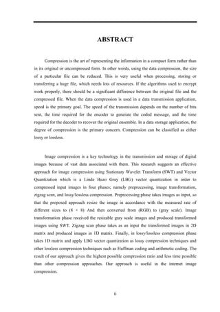
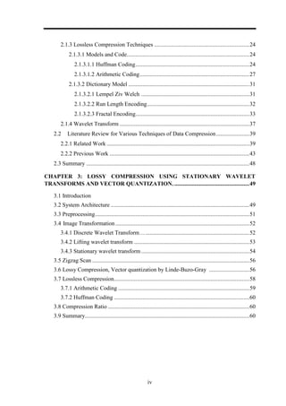
Vector Quantization (VQ) is a block-coding technique that quantizes blocks of data
instead of single samples. VQ exploits the correlation between neighboring signal samples
by quantizing them together. VQ Compression contains two components: VQ encoder and
decoder as shown in Figure 1.1. At the encoder, the input image is portioned into a set of
non-overlapping image blocks. The closest code word in the code book is then found for
each image block. Here, the closest code word for a given block is the one in the code book
that has the minimum squared Euclidean distance from the input block. Next, the
corresponding index for each searched closest code word is transmitted to the decoder.
Compression is achieved because the indices of the closest code words in the code book
sent to the decoder instead of the image blocks themselves [7].

18. Chapter 1 Introduction
3
Vector quantization (VQ) is a powerful method for image compression due to its
excellent rate-distortion performance and its simple structure. Some efficient clustering
algorithms are developed based on the VQ-like approach. However, the VQ algorithm still
employs a full search method to ensure the best-matched code word and consequently
results in the computational requirement is large. Therefore, many research efforts were
paid on simplifying the search complexity for the encoding process. These approaches are
further classified into two types in terms of simplified technique. One is the tree-structured
VQ (TSVQ) techniques, and the other is the triangular inequality elimination (TIE) based
approaches [8].
Figure 1.1: Vector quantization encoder and decoder
This thesis focuses on lossy compression because it is the most popular category in
real applications.
1.1 Lossy Compression
Lossy compression works very differently. These programs simply eliminate
"unnecessary" bits of information, tailoring the file so that it is smaller. This type of
compression is used a lot for reducing the file size of bitmap pictures, which tend to be
fairly bulky [9]. This may examine the color data for a range of pixels, and identifies subtle
variations in pixel color values that are so minute that the human eye/brain is unable to

19. Chapter 1 Introduction
4
distinguish the difference between them. The algorithm may choose a smaller range of
pixels whose color value differences fall within the boundaries of our perception, and
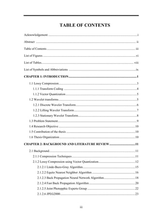
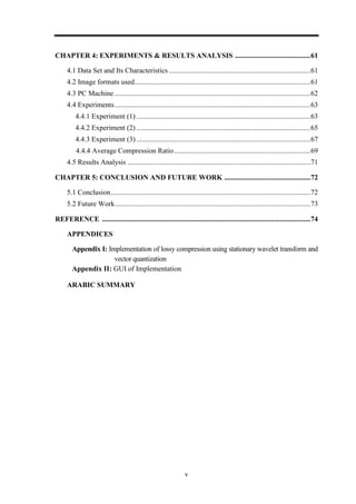
substitute those for the others. The Lossy compression framework is shown in Figure (1.2).
Figure 1.2: Lossy compression framework
To achieve this goal one of the following operations is performed. 1. Predicted image
is formed by predicting pixels based on the values of neighboring pixels of the original
image. Then the residual image is formed which is the difference between the predicted
image and the original image. 2. Transformation a reversible process that reduces
redundancy and/or provides an image representation that is more amenable to the efficient
extraction and coding of relevant information. 3. Quantization process compresses a range
of values to a single quantum value. When the number of discrete symbols in a given
stream is reduced, the stream becomes more compressible. Entropy coding is then applied
to achieve further compression. Major performance considerations of a lossy compression
scheme are: a) the compression ratio (CR), the signal-to noise ratio (PSNR) of the
reconstructed image with respect to the original, and c) the speed of encoding and
decoding [9].
We will use the following techniques in the Lossy compression process:
1.1.1 Transform Coding
Transform coding algorithm usually start by partitioning the original image into sub
images (blocks) of small size (usually 8 x 8). For each block the transform coefficients are
calculated, effectively converting the original 8 x 8 array of pixel values into an array of
coefficients closer to the top-left corner usually contains most of the information needed to
quantize and encode the image with little perceptual distortion. The resulting coefficients
Original Image
Data
Prediction/Transformat
ion/ Decomposition
Quantization
Modeling and
Encoding
Compressed Image

20. Chapter 1 Introduction
5
are then quantized and the output of the quantized issued by a symbol encoding technique
to produce the output bit stream representing the encoded image [9].
1.1.2 Vector Quantization
The vector quantization is a classical quantization technique for signal processing
and image compression, which allows the modelling of probability density functions by the
distribution of prototype vectors. The main use of vector quantization (VQ) is for data
compression [10] and [11]. It works by dividing a large set of values (vectors) into groups
having approximately the same number of points closest to them. Each group is
represented by its centroid value, as in LBG algorithm and some other algorithms [12].
The density matching property for vector quantization is powerful, especially in the
case for identifying the density of large and high dimensioned data. Since data points are
represented by their index to the closest centroid, commonly occurring data have less error
and rare data have higher error. Hence VQ is suitable for lossy data compression. It can
also be used for lossy data correction and density estimation. The methodology of vector
quantization is based on the competitive learning paradigm, hence it is closely related to
the self-organizing map model. Vector quantization (VQ) is used for lossy data
compression, lossy data correction and density estimation [12].
Our approach is considered a lossy compression technique that enhances lossy
compression technique by using stationary wavelet transform and vector quantization to
solve the major problems of lossy compression techniques.
1.2 Wavelet Transforms (WT)
Wavelets are signals which are local in time and scale and generally have an
irregular shape. A wavelet is a waveform of effect limited duration that has an average
value of zero. The term „wavelet‟ comes from the fact that they integrate to zero; they
wave up and down across the axis. Many wavelets also display a property ideal for
compact signal representation: orthogonally. This property ensures that data is not over
represented. A signal can be decomposed into many shifted and scaled representations of
the original mother wavelet. A wavelet transform can be used to decompose a signal into
component wavelets. Once this is done the coefficients of the wavelets can be decimated to

21. Chapter 1 Introduction
6
remove some of the details. Wavelets have the great advantage of being able to separate
the fine details in a signal. Very small wavelets can be used to isolate very fine details in a
signal, while very large wavelets can identify coarse details. In addition, there are many
different wavelets to choose from. Various types of wavelets are: Morlet, Daubechies, etc.
One particular wavelet may generate a more sparse representation of a signal than another,
so different kinds of wavelets must be examined to see which is most suited to image
compression [13].
1.2.1 Discrete Wavelet Transform (DWT)
The Discrete Wavelet Transform (DWT) of image signals produces a no redundant
image representation, which provides better spatial and spectral localization of image
formation, compared with other multi scale representations such as Gaussian and Laplacian
pyramid. Recently, Discrete Wavelet Transform has attracted more and more interest in
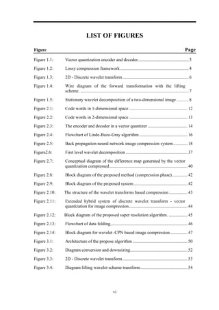
image fusion. An image can be decomposed into a sequence of different spatial resolution
images using DWT. In case of a 2D image, an N level decomposition can be performed,
resulting in 3N+1 different frequency bands and it is shown in Figure 1.3 Optimal
decomposition level of the discrete, stationary, and dual tree complex [14].
Figure 1.3: 2D-Discrete wavelet transforms

22. Chapter 1 Introduction
7
1.2.2 Lifting Wavelet Transform (LWT)
The lifting scheme (LS) has been introduced for the efficient computation of DWT
.For image compression, it is very necessary that the selection of transform should reduce
the size of the resultant data as compared to the original data set .So a new lossless image
compression method is proposed. Wavelet using the lifting scheme significantly reduces
the computation time, speed up the computation process. The lifting transforms even at its
highest level is very simple. The lifting transform can be performed via two operations:
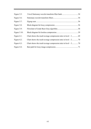
Split, Predict and Update [15]. Suppose we have the one dimensional signal a0. The
Lifting is done by performing the following sequence of operations:
1.Split a0 into Even-1 and Odd-1
2. d-1 = Odd-1 – Predict (Even-1)
3. a-1 = Even-1 + Update( d-1 )
These steps are repeated to construct multiple scales of the transform. The wiring
diagram in Figure 1.4 shows the forward transform visually. The coefficients “a” are
representing the averages in the signal that is Approximation coefficient, while the
coefficients in “d” represent the differences in the signal that is Detailed Coefficient. Thus,
these two sets also correspond to the low- pass and high- pass frequencies present in the
signal [16].
Figure 1.4: Wire diagram of forward transformation with the lifting scheme

23. Chapter 1 Introduction
8
1.2.3 Stationary Wavelet Transform (SWT)
Among the different tools of multi-scale signal processing, wavelet is a time-frequency
analysis that has been widely used in the field of image processing such as denoising,
compression, and segmentation. Wavelet-based denoising provides multi-scale treatment of
noise, down-sampling of sub-band images during decomposition and the thresholding of wavelet
coefficients may cause edge distortion and artifacts in the reconstructed images. To improve the
limitation of the traditional wavelet transform, a multi-layer stationary wavelet transform (SWT)
was adopted in this study, as illustrated in Figure 1.5.
In Figure 1.5, Hj and Lj represent high-pass and low-pass filters at scale j, resulting
from the interleaved zero padding of filters Hj-1 and Lj-1 (j>1). LL0 is the original image
and the output of scale j, LLj, would be the input of scale j+1. LLj+1 denotes the low-
frequency (LF) estimation after the stationary wavelet decomposition, while LHj+1, HLj+1
and HHj+1 denote the high frequency (HF) detailed information along the horizontal,
vertical and diagonal directions, respectively [5].
Figure 1.5: Stationary wavelet decomposition of a two-dimensional image

24. Chapter 1 Introduction
9
These sub-band images would have the same size as that of the original image
because no down-sampling is performed during the wavelet transform. In this study, the
Haar wavelet was applied to perform multi-layer stationary wavelet transform on a 2D
image. Mathematically, the wavelet decomposition is defined as:
LLj+1(χ, γ) = L[n] L [m] LLj (2j+1 m- χ, 2j+1 n- γ)
LHj+1(χ, γ) = L[n] H [m] LLj (2j+1 m- χ, 2j+1 n- γ)
HLj+1(χ, γ) = H[n] L [m] LLj (2j+1 m- χ, 2j+1 n- γ)
HHj+1(χ, γ) = H[n] H [m] LLj (2j+1 m- χ, 2j+1 n- γ)
Where L[·] and H[·] represent the low pass and high pass filters respectively, and
LL0(X,Y)=F(X,Y)
Compare with the traditional wavelet transform, the SWT has several advantages.
First, each sub-band has the same size, so it is easier to get the relationship between the
sub-bands. Second, the resolution can be retained since the original data is not decimated.
Also at the same time the wavelet coefficients contain much redundant information which
helps to distinguish the noise from the feature. In this study, the image processing and
stationary wavelet transform are performed using MATLAB programming language. The
proposed method is tested using Standard images as well as image sets selected from Heath
et al.‟s library. For the sake of thoroughness, the developed method is compared with the
standard Sobel, Prewitt, Laplacian, and Canny edge detectors [5].
1.3 Problem Statement
The large increase in the data lead to delays in access to the information required and
this leads to a delay in the time. Large data lead to data units and storage is full this leads
to the need to buy a bigger space for storage and losing money. Large data lead to give
inaccurate results for the similarity of data and this leads to getting inaccurate information.
Also to show the difference between the types of transforms Stationary Wavelet
Transforms and Discrete Wavelet Transform and Lifting Wavelet Transform because they
are very similar at one level so we used three levels.
(1.1)

25. Chapter 1 Introduction
10
1.4 Research Objective
In lossy compression, the compression ratio is unaccepted. The proposed system
suggests an image compression method of lossy image compression through the three
types of transformations such as stationary wavelet transform, discrete wavelet transforms,
and lifting wavelet transform and the comparison between the three types and the use of
vector quantization (VQ) to improve the image compression process.
1.5 Contribution of the thesis
Our thesis has two contributions. The first contribution is the lossy compressed
approach using stationary wavelet transforms and vector quantization has less compressed
data than other wavelet transformation such as discrete wavelet transform and lifting
wavelet transform. The second conclusion, when apply lossless compressors of the type of
the arithmetic coding and Huffman encoding, the size of compressed data by arithmetic
coding is better than Huffman coding.
Our approach built to compress the data by using stationary wavelet transform
(SWT) and vector quantization (VQ) and arithmetic coding.
1.6 Thesis Organization
Chapter two introduces the details chapter illustrating previous studies on image
compression and the techniques used. Chapter three describes in detail the proposed
system and how it improves the image compression with the lossy image compression
technologies and lossless image compression techniques. Chapter four introduces the
empirical results that applied on the proposed system, its effectiveness, and an analysis of
results. It also compares between the results of the Used for a number of techniques as
used in the image compression. Chapter five gives a general summary of the thesis, the
research conclusions, and the top recommendations the researcher believes will be
necessary for future research.

26. Chapter 2 Background and Literature Review
11
BACKGROUND AND LITERATURE REVIEW
This chapter offers some important background related to the proposed system that
including wavelet transform and vector quantization. It also introduces a taxonomy of
image compression techniques, and covers a literature review on image compression
algorithms.
2.1 Background
2.1.1 Compression Techniques
Compression techniques come in two forms: lossy and lossless. Generally a lossy
technique means that data are saved approximately rather than exactly. In contrast lossless
techniques save data exactly. They look for sequences that are identical and code these.
This type of compression has a lower compression rate than a lossy technique, but when
the file is recovered it is identical to the original. Generally speaking, Lossless data
compression is used as a component within lossy data compression technologies. Lossless
compression is used in cases where it is important that the original and the decompressed
data be identical, or where deviations from the original data could be deleterious. Typical
examples are executable programs, text documents, and source code. Lossless compression
methods may be categorized according to the type of data they are designed to compress.
While, in principle, any general-purpose lossless compression algorithm can be used on
any type of data, many are unable to achieve significant compression on data that are not
of the form for which they were designed to compress [18].
In lossless compression schemes, the reconstructed image, after compression, is
numerically identical to the original image. However, lossless compression can only
achieve a modest amount of compression. An image reconstructed following lossy
compression contains degradation relative to the original. Often this is because the
compression scheme completely discards redundant information. However, lossy schemes
are capable of achieving much higher compression. Under normal viewing conditions, no
visible loss is perceived (visually lossless). Table 1 describes the comparison between
loosy and lossless compression in some items [17].

27. Chapter 2 Background and Literature Review
12
Table 2.1: Comparison between lossy and lossless compression techniques
Item Lossy Compression Lossless Compression
Reconstructed image
Contains degradation relative to
the original image.
Numerically identical to the
original image.
Compression rate
High compression (visually
lossless).
2:1 (at most 3:1).
Application
Music, photos, video, medical
images, scanned documents, fax
machines.
Databases, emails,
spreadsheets, office
documents, source code.
2.1.2 Lossy Compression Vector Quantization
Figure 2.1: Code words in 1-dimensional space
Vector quantization (VQ) is a lossy data compression method based on the principle
of block coding. It is a fixed-to-fixed length algorithm. A VQ is nothing more than an
approximate. The idea is similar to that of “rounding-off” (say to the nearest integer) [21]
and [22]. The following example shown in Figure 2.1 represents every number less than -2
is approximated by -3, all numbers between -2 and 0 are approximated by -1, every
number between 0 and 2 are approximated by +1, and every number greater than 2 are
approximated by +3. The approximate values are uniquely represented by 2 bits. This is a
1-dimensional, called 2-bit VQ. It has a rate of 2 bits/dimension. In the above example, the
stars are called code vectors [21].
A vector quantizer map k-dimensional vectors in the vector space a finite set of
vectors Y = {y: i = 1, 2, ... , N}. Each vector is called a code vector or a code word, and
the set of all the codewords is called a codebook. Associated with each codeword is a
nearest neighbor region called encoding region or Voronoi region [21] and [23] and it is
defined by:
| || || } ................................... (1)

28. Chapter 2 Background and Literature Review
13
The set of encoding region's partition, the entire space such that:
⋃ ⋂ .......................... (2)
Thus the set of all encoding regions is called the partition of the space. In the
following example, we take vectors in the two dimensional case without loss of generality
in Figure 2.1 In the figure, Input vectors are marked with an x, code words are marked with
solid circles, and the Voronoi regions are separated with boundary lines. The figure shows
some vectors in space. Associated with each cluster of vectors is a representative code
word. Each code word resides in its own Voronoi region. These regions are separated by
imaginary boundary lines in Figure 2.2 given an input vector; the code word that is chosen
to represent it is the one in the same Voronoi region. The representative code word is
determined to be the closest in Euclidean distance from the input vector [21].
The Euclidean distance is defined by:
√∑ ....................................... (3)
Where is the component of the input vector, and is the component of the
code word . In Figure 2.2 there are 13 regions and 13 solid circles, each of which can be
uniquely represented by 4 bits. Thus, this is a 2-dimensional, 4-bit VQ. Its rate is also 2
bits/dimension [21].
Figure 2.2: Code words in 2-dimensional space

29. Chapter 2 Background and Literature Review
14
A vector quantizer is composed of two operations. The first is the encoder, and the
second is the decoder [24]. The encoder takes an input vector and outputs the index of the
code word that offers the lowest distortion. In this case the lowest distortion is found by
evaluating the Euclidean distance between the input vector and each code word in the
codebook. Once the closest code word is found, the index of that code word is sent through
a channel (the channel could be computer storage, communications channel, and so on).
When the decoder receives the index of the code word, it replaces the index with the
associated code word. Figure 2.3 shows a block diagram of the operation of the encoder
and the decoder [21].
Figure 2.3: The Encoder and decoder in a vector quantizer
In Figure 2.3, an input vector is given, the closest code word is found and the index
of the code word is sent through the channel. The decoder receives the index of the code
word, and outputs the code word [21].
The drawback of vector quantization, this technique generates code book in very
slow speed than bpp [25].

30. Chapter 2 Background and Literature Review
15
2.1.2.1 Linde-Buzo-Gray Algorithm:
Generalized Lloyd Algorithm (GLA), which is also called, Linde-Buzo-Gray (LBG)
Algorithm They used a mapping function to partition training vectors in N clusters. The
mapping function is defined as in [10].
→ CB
Let X = (x1, x2,…,xk) be a training vector and d(X, Y) be the Euclidean Distance
between any two vectors. The iteration of GLA for a codebook generation is given as
follows:
1. LBG algorithm
Step 1: Randomly generate an initial codebook CB0.
Step 2: i = 0.
Step 3: Perform the following process for each training vector.
Compute the Euclidean distances between the training vector and the
code words in . The Euclidean distance is defined as
∑ ................................... (4)
Search the nearest code word among .
Step 4: Partition the codebook into N cells.
Step 5: Compute the centroid of each cell to obtain the new codebook CBi+1.
Step 6: Compute the average distortion for CBi+1. If it is changed by a small
enough amount since the last iteration, the codebook may converge and
the procedure stops. Otherwise, i = i + 1 and go to Step 3 [10].
LBG algorithm has the local optimization problem and the utility of each codeword
in the codebook is low. The local optimization problem means that the codebook
guarantees local minimum distortion, but not global minimum distortion [29].

31. Chapter 2 Background and Literature Review
16
Figure 2.4: Flowchart of Linde-Buzo-Gray Algorithm
2.1.2.2 Equitz Nearest Neighbor
The selection of initial codebook by the LBG algorithm is poor, which results in an
undesirable final codebook. Another algorithm Equitz Nearest neighbor (ENN) is used in
which no need for selection of initial codebook. As the beginning of ENN algorithm, all
training vectors are viewed as initial clusters (code vectors). Then, the two nearest vectors
are found and merged by taking their average. A new vector is formed which replaces and
reduce the number of clusters by one. The Process is going on until desired number of
clusters is not obtained [30].
The steps for the implementation of the ENN algorithm are as follows:
2. ENN Algorithm
1. Initially, all the image vectors taken as the initial codewords.
2. Find each of two nearest codewords by the equation:

32. Chapter 2 Background and Literature Review
17
Od (X, Yi) =k-1Σj=0|Xj–Yi, j|............................... (2.2)
Where “X” represents an input vector from the original image and “Y”
represents a codeword, and merge them by taking their average where “k”
represents the codeword length.
3. The new codeword replaces the two codeword and reduce the number of
codewords by one.
4. Repeat step 2 and step 3 until desired number of codewords is reached. The ENN
requires a long time and large number of iterations to design the codebook.
Therefore, to decrease the number of iterations and time required to generate the
codebook, an image block distortion threshold value (dth) is calculated [10].
The ENN algorithm is modified as:
1. Determine the desired number of codeword and the maximum number of gray
levels in the image (max–gray)
2. Distortion threshold (dth) is calculated as:
dth=k× (max-gray/64) ..................................... (5)
Where „k‟ is codeword length
3. Calculate the distortion error between a taken codeword and a next codeword. If
the distortion error is less than or equal to dth, then merge these two codeword
and reduce the number of codeword by one. Otherwise, consider the next
codeword.
4. Repeat the step 3 until we obtain the number of codewords equal to desired
number of codewords.
5. Even, after all the codewords are compared and merged, the resultant number of
codewords greater than desired number of codewords, then change the dth value
as follows
Dth=dth+k×(max-gray/256) .................................. (6)
And then go to step 3.

33. Chapter 2 Background and Literature Review
18
2.1.2.3 Back Propagation Neural Network Algorithm
BPNN algorithm helps to increase the performance of the system and to decrease the
convergence time for the training of the neural network [31]. BPNN architecture is used
for both image compression and also for improving VQ of images. A BPNN consists of
three layers: input layer, hidden layer and output layer. The number of neurons in the input
layer is equal to the number of neurons in the output layer. The number of neurons in the
hidden layer should be less than that of the number of neurons in the input layer. Input
layer neurons represent the original image block pixels and output layer neuron represents
the pixels of the reconstructed image block. The assumption in hidden layer neurons is that
the arrangement is in one-dimensional array of neurons, which represents the element of
codeword. This process produces an optimal VQ codebook. The source image is divided
into non-overlapping blocks of pixels such that block size equals the number of input layer
neurons and the number of hidden layer neurons equals the codeword length. In the BP
algorithm, to design the codebook, the codebook is divided into rows and columns in
which rows represent the number of patterns of all images and columns represents the
number of hidden layer units [10].
Figure 2.5: Back propagation neural network image compression system
The implementation of BPNN VQ encoding can be summarized as follows:

34. Chapter 2 Background and Literature Review
19
2. BPNN algorithm
1. Divide the source image into non-overlapping blocks with predefined block
dimensions (P), where (P×P) equals the number of neurons in the input layer.
2. Take one block from the image, normalize it, convert the image into pixels
(rasterizing), and apply it to the input layer neurons of BPNN.
3. Execute one iteration BP in the forward direction to calculate the output of
hidden layer neurons.
4. From the codebook file, find the codeword that best matches the outputs of
hidden layer neurons.
5. Store index i.e. position of this codeword in codebook in the compressed version
of source image file.
6. For all the blocks of source image, repeat the steps from step2 to step5 [10].
Number of bits required for indexing each block equals to log2M, where M is
codebook length.
The implementation of BPNN VQ decoding process can be described as follows:
1. Open compressed VQ file
2. Take one index from this file.
3. This index is then replaced by its corresponding codeword which is obtained
from the codebook and this codeword is assumed to be the output of hidden layer
neurons.
4. Execute one iteration BP in the forward direction to calculate the output of the
output layer neurons, then de-rasterizing it, de-normalize it and store this output
vector in a decompressed image file.
5. Repeat steps from step2 to step4 until the end of the compressed file.
The BP algorithm is used to train the BPNN network to obtain the codebook with
smaller size with improved performance of the system. The BPNN image compression
system has the ability to decrease the errors that occur during transmission of compressed
images through analog or digital channel. Practically, we can note that BPNN has the
ability to enhance any noisy compressed image that has been corrupted during compressed
image transmission through a noisy digital or analog channel. BPNN has the capacity to

35. Chapter 2 Background and Literature Review
20
compress untrained images, but not in the same performance of trained images. This can be
done, especially when using a small number of image block dimension [33].
2.1.2.4 Fast Back Propagation Algorithm
The FBP algorithm is used for training the designed BPNN to reduce the
convergence time of BPNN as possible as. The fast back propagation (FBP) algorithm is
based on the minimization of an objective function after initial adaption cycles. This
minimization can be obtained by reducing lambda (λ) from unity to zero during network
training. The FBP algorithm differs from standard BP algorithm in the development of
alternative training criterion. This criterion indicates that (λ) must change from 1 to 0
during training process i.e. λ approaches to zero as total error decreases. In each adaption
cycle, λ should be calculated from the total error at that point, according to the equation:
λ=λ (E), where E is error of network, indicates that λ≈1 when E˃˃1.When E˃˃1 for any
positive integer n, 1/En approaches zero, therefore exp(-1/En) ≈1. When E˂˂1, 1/En is
very large, therefore exp(-1/En)≈0. As a result, for the reduction of λ from 1 to 0, a suitable
rule is as follows [32]:
λ=λ(E)= exp (-μ/En).....................................(7)
Where μ is a positive real number and n is a positive integer. When n is small,
reduction of λ is faster, when E˃˃1. It has been experimentally verified that if λ is much
smaller than unity during initial adaption cycles, algorithm may be trapped in local
minimum. So, n should be greater than 1.
Thus, λ is calculated during any network training according to equ. 6[32]:
λ = λ(E)=exp(-μ/E2).......................................(8)
In the FBP algorithm, all the hidden layer neurons and output layer neurons use
hyperbolic tangent function instead of sigmoid functions in the BPNN architecture. So, the
equation is modified for hyperbolic tangent function as follows [32]:
F (NET j)= ( J - J) / ( J - J)............... (9)
And derivative of this function is as follows:
F‫(׳‬NET j)=(1-(F(NETj)2).........................................(10)
So that F (NET j) lies between -1 and 1.

36. Chapter 2 Background and Literature Review
21
Table 2.2 compares the previous algorithm for some parameters such as code book
size, code word size, storage capacity, code generation time, complexity time, and
performance.
Table 2.2: Comparison of various algorithms of vector quantization
Parameters LBG ENN BPNN FBP
Codebook size
Very large
super
codebook
Small codebook as
compared to LBG
algorithm.
Codebook with
smaller size as
compared to
ENN algorithm
Codebook size is same
as that of BPNN
algorithm.
Codeword size
The size of
each
codeword in
the codebook
is P×P, where
P is the
dimension of
image block.
The size of
codeword in the
codebook is P×P,
where P is the
dimension of image
block
The size of each
codeword in the
codebook is
equal to the
number of
hidden layer
neurons.
The size of each
codeword is same as
BPNN algorithm
Storage space
It requires
more storage
space for the
codebook.
It requires less
storage space for
the codebook
It requires less
storage space as
compared to
ENN algorithm.
It requires same storage
space as that of BPNN
algorithm
Codebook
generation time
It takes long
time for the
generation of
the codebook.
It takes less time
for the generation
of the codebook.
It takes less time
for the
generation of the
codebook as
compare to ENN
It takes less time for the
generation of codebook
than BPNN algorithm
Complexity time
A complete
design
requires a
large number
of
computations
This algorithm
reduces the
computations
dramatically
Computational
load is less for
encoding and
decoding
process as
compared to
ENN algorithm
Computational load is
less for encoding and
decoding process as
compared to ENN
algorithm
Convergence
time
Convergence
time is very
large
Convergence time
is less than the
LBG algorithm
Convergence
time is less than
that of the ENN
algorithm.
FBP trains the BPNN
image compression
system to speed up the
learning process and
reduce the convergence
time
Performance
The
performance
of this
algorithm is
not so good.
Performance is
better than LBG
algorithm as LBG
selects the initial
codebook randomly
Performance is
far much better
than ENN
algorithm
Performance is better
than BPNN algorithm

37. Chapter 2 Background and Literature Review
22
2.1.2.5 Joint Photopphic Experts Group
JPEG stands for Joint Photopphic Experts Group, it is indeed one of the most used
standards in the field of the compression of photographic images and it was created at the
beginning of the 90s. It tums out moreover very competitive when it is used in a weak or
an average compression ratios. But the mediocre quality of the obtained images in a higher
compression ratio as well as its lack of flexibility and features gave a clear evidence of its
incapability to satisfy all the application requirements in the field of the digital image
processing. Based on those facts, members of the PEG group recovered to develop a new
standard for image coding offering more flexibility and functionalities: JPEG2000 [69].
2. Joint Photopphic Experts Group (JPEG) Algorithm
The algorithm behind JPEG is relatively straightforward and can be explained
through the following steps [70]:
1. Take an image and divide it up into 8-pixel by 8-pixel blocks. If the image
cannot be divided into 8-by-8 blocks, then you can add in empty pixels around
the edges, essentially zero-padding the image.
2. For each 8-by-8 block, get image data such that you have values to represent the
color at each pixel.
3. Take the Discrete Cosine Transform (DCT) of each 8-by-8 block.
4. After taking the DCT of a block, matrix multiply the block by a mask that will
zero out certain values from the DCT matrix.
5. Finally, to get the data for the compressed image, take the inverse DCT of each
block. All these blocks are combined back into an image of the same size as the
original.
As it may be unclear why these steps result in a compressed image, I'll now explain
the mathematics and the logic behind the algorithm [70].

38. Chapter 2 Background and Literature Review
23
2.1.2.6 JPEG2000
A. Historic : With the continual expansion of multimedia and Internet applications, the
needs and requirements of the technologies used, grew and evolved In March 1997 a
new call for contributions were launched for the development of a new standard for the
compression of still images, the JPEG2000 [69]. This project, JTC2 1.29.14 (15444),
was intended to create a new image coding system for different types of still images
(bi-level, gray-level, color, multicomponent). The standardization process, which is
coordinated by the JTCI/SC29/WGI of ISO/lEC3, has produced the Final Draft
International Standard (FDIS') in August 2000. The International Standard (Is) was
ready by December 2000. Only editorial changes are expected at this stage and
therefore, there will be no more technical or functional changes in Part 1 of the
Standard
B. Characteristics and features: The purpose of having a new standard was twofold.
First, it would address a number of weaknesses in the existing standard second, it
would provide a number of new features not available in the JPEG standard The
preceding points led to several key objectives for the new standard, namely that it
should enclose [69]:
1) Superior low bit-rate performance,
2) Lossless and lossy compression in a single code-stream,
3) Continuous-tone and bi-level compression,
4) Progressive transmission by pixel accuracy and resolution,
5) Fixed-rate, fixed-size,
6) Robustness to bit errors,
7) Open architecture,
8) Sequential build-up capability,
9) Interface with MPEG-4,
10) Protective image security,
11) Region of interest

39. Chapter 2 Background and Literature Review
24
2.1.3 Lossless Compression Techniques
The extremely fast growth of data that needs to be stored and transferred has given
rise to the demands of better transmission and storage techniques. Lossless data
compressions categorized into two types are: models & code and dictionary models.
Various lossless data compression algorithms have been proposed and used. Huffman
Coding, Arithmetic Coding, Shannon Fano Algorithm, Run Length Encoding Algorithm
are some of the techniques in use [34].
2.1.3.1 Models and Code
Model code divided to Huffman coding and Arithmetic coding
2.1.3.1.1 Huffman Coding
A first Huffman coding algorithm was developed by David Huffman in 1951.
Huffman coding is an entropy encoding algorithm used for lossless data compression. In
this algorithm fixed length codes are replaced by variable length codes. When using
variable-length code words, it is desirable to create a prefix code, avoiding the need for a
separator to determine codeword boundaries. Huffman Coding uses, such prefix code [34].
Huffman procedure works as follow:
1. Symbols with a higher frequency are expressed using shorter encodings than
symbols which occur less frequently.
2. The two symbols that occur least frequently will have the same length.
The Huffman algorithm uses the greedy approach i.e. at each step the algorithm
chooses the best available option. A binary tree is built up from the bottom up.
To see how Huffman Coding works, let‟s take an example. Assume that the
characters in a file to be compressed have the following frequencies:
A: 25 B: 10 C: 99 D: 87 E: 9 F: 66
The processing of building this tree is:
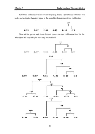
Create a list of leaf nodes for each symbol and arrange the nodes in the order from
highest to lowest.
C: 99 D:87 F:66 A:25 B:10 E:9

40. Chapter 2 Background and Literature Review
25
Select two leaf nodes with the lowest frequency. Create a parent node with these two
nodes and assign the frequency equal to the sum of the frequencies of two child nodes.
Now add the parent node in the list and remove the two child nodes from the list.
And repeat this step until you have only one node left.

41. Chapter 2 Background and Literature Review
26
Now label each edge. The left child of each parent is labeled with the digit 0 and
right child with 1. The code word for each source letter is the sequence of labels along the
path from root to the leaf node representing the letter.
Huffman Codes are shown below in the table [34].
Table 2.3: Huffman Coding
C 00
D 01
F 10
A 110
B 1110
E 1111
2. Huffman Encoding Algorithm
Huffman Encoding Algorithm [52].
Huffman (W, n) //Here, W means weight and n is the no. of inputs
Input: A list W of n (Positive) Weights.
Output: An Extended Binary Tree T with Weights Taken from W that gives the
minimum weighted path length.
Procedure: Create list F from singleton trees formed from elements of W.
While (F has more than 1 element) do
Find T1, T2 in F that have minimum values associated with their roots // T1 and T2
are sub tree .
Construct new tree T by creating a new node and setting T1 and T2 as its children
Let, the sum of the values associated with the roots of T1 and T2 be associated with
the root of T Add T to F
Do Huffman-Tree stored in the F

42. Chapter 2 Background and Literature Review
27
2.1.3.1.2 Arithmetic Coding
Arithmetic coding (AC) is a statistically lossless encoding algorithm with very high
compression efficiency and is especially useful when dealing with the source with an
alphabet of small size. Nowadays, AC is widely adopted in the image and video coding
standards, such as JPEG2000 [22] and [39]. Recent researches on secure arithmetic coding
primary focus on the two approaches: the interval splitting AC (ISAC) and the randomized
AC (RAC). In [40] and [41], the strategy of key-based interval splitting had been
successfully incorporated with arithmetic coding to construct a novel coder with the
capabilities of compression and encryption. This approach has been studied deeply just for
the floating-point arithmetic coding over the past few years. On compression efficiency,
the authors illustrated that even the interval is just split (the total length kept unchanged) in
an arithmetic coder, the code length will raise a little relative to the floating-point
arithmetic coding [42] analyzed that the key-based interval splitting AC is vulnerable to
known-plaintext attacks [43]. Further used message in distinguishability to prove that
ISAC is still insecure under [36].
Cipher text-only attacks even under the circumstance that different keys are used to
encrypt different messages. In order to enhance the security, [44] provided an extended
version of ISAC, called Secure Arithmetic Coding (SAC), which applies two permutations
to the input symbol sequence and the output codeword. However,[45] and [46]
independently proved that it is still not secure under the chosen-plaintext attacks and
known-plaintext attacks due to the regularities of permutations steps [47] presented a
randomized arithmetic coding (RAC) algorithm, which achieves the capability of
encryption by randomly swapping two symbol intervals during the process of binary AC.
Although RAC does not suffer any loss of compression efficiency, its security problem
does exist [48] proved that it is vulnerable to cipher-only attacks.
Recently [49] presented a secure integer AC scheme (here called MIAC) that performs
the compression and the encryption simultaneously. In this scheme, the size ratio D𝛼1,+1/λn of
interval allocated to the symbol 𝛼1 will be far approximated to the probability P(𝛼1) and the
size ratios D𝛼1,n+1/λn of interval allocated to the symbol 𝛼i will be far approximated to the
probability P(𝛼i). In this paper, we further try to propose another secure arithmetic coding
scheme with good compression efficiency and highest secrecy.

43. Chapter 2 Background and Literature Review
28
Illustrated Example of Arithmetic Encoding
Arithmetic Coding works, let‟s take an example, we have a string:
BE_A_BEE
And we now compress it using arithmetic coding.
Step 1: in the first step we do is look at the frequency count for the different letters:
E B _ A
3 2 2 1
Step 2: In the second step we encode the string by dividing up the interval [0, 1] and
allocate each letter an interval whose size depends on how often it count in the string. Our
string start with a‟B‟, so we take the „B‟ interval and divide it up again in the same way:
The boundary between „BE‟ and „BB‟ is 3/8 of the way along the interval, which is
itself 2/3 long and starts at 3/8. So boundary is 3/8 + (2/8) * (3/8) = 30/64. Similarly the
boundary between „BB‟ and „B_‟ is 3/8+ (2/8) * (5/8) = 34/64, and so on. [51].
Step 3: In the third step we see next letter is now „E‟, so now we subdivide the”E‟
interval in the same way. We carry on through the message….And, continuing in this way,
we eventually obtain:

44. Chapter 2 Background and Literature Review
29
And continuing in this way, we obtain:
So we represent the message as any number in the interval
[7653888/16777216, 7654320/16777216]
However, we cannot send numbers like 7654320/16777216 easily using a computer.
In decimal notation, the rightmost digit to the left of the decimal point indicates the number
of units; the one to its left gives the number of tens: the next one along gives the number of
hundred, and so on.
7653888 = (7*106) + (6*105) + (5*104) + (3*103) + (8*102) + (8*10) + 8
Binary numbers are almost exactly the same, we only deal with powers of 2 instead
of power of 10. The rightmost digit of a binary number is unitary (as before) the one to its
left gives the number of 2s, the next one the number of 4s, and so on.
110100111 = (1*28) + (1*27) + (0*26) + (1*25) + (0*24) + (0*23) + (1*22) +
(1*21) + 1 = 256 + 128 + 32 + 4 + 2 + 1 = 423 in denary (i.e. base 10) [51].

45. Chapter 2 Background and Literature Review
30
2. Arithmetic Encoding Algorithm
BEGIN
low = 0.0; high = 1.0; range = 1.0;
While (symbol i= terminator)
{
get (symbol) ;
Low = low + range * Range_low (symbol);
Low = low + range * Range_high (symbol);
range = high – low;
}
Output a code so that low <= code < high;
END
Huffman Coding Algorithm uses a static table for the whole coding process, so it is
faster. However, it does not produce efficient compression ratios. On the contrary,
Arithmetic algorithm can generate a high compression ratio, but its compression speed is
slow [34]. Table 2.4 presents a simple comparison between these compression methods.
Table 2.4: Huffman coding vs. Arithmetic coding
Compression Method Arithmetic Huffman
Compression ratio Very good Poor
Compression speed Slow Fast
Decompression speed Slow Fast
Memory space Very low Low
Compressed pattern matching No Yes
Permits Random access No Yes
Input Variable Fixed
Output Variable Variable

46. Chapter 2 Background and Literature Review
31
2.1.3.2 Dictionary Model
Dictionary model divided to Lempel Ziv Welch, Run length encoding and Fractal
encoding
2.1.3.2.1 Lempel Ziv Welch :
Lempel–Ziv–Welch Coding: Lempel–Ziv–Welch (LZW) is a universal lossless data
compression algorithm created by Abraham Lempel, Jacob Ziv, and Terry Welch. It was
published by Welch in 1984 as an improved implementation of the LZ78 algorithm
published by Lempel and Ziv in 1978. LZW is a dictionary based coding. Dictionary based
coding can be static or dynamic. In the static dictionary coding, the dictionary is fixed
when the encoding and decoding processes. In dynamic dictionary coding, dictionary is
updated on the fly. The algorithm is simple to implement, and has the potential for very
high throughput in hardware implementations. It was the algorithm of the widely used
UNIX file compression utility compress, and is used in the GIF image format. LZW
compression became the first widely used universal image compression method on
computers. A large English text file can typically be compressed via LZW to about half its
original size [35].
3. LZW Encoding Algorithm
LZW Encoding Algorithm [52].
Step 1: At the start, the dictionary contains all possible roots, and P is empty;
Step 2: C: = next character in the char stream;
Step 3: Is the string P+C present in the dictionary?
(a) if it is, P := P+C (extend P with C);
( b) if not,
– output the code word which denotes P to the code stream;
– add the string P+C to the dictionary;
– P := C (P now contains only the character C); (c) Are there more
characters in the char stream?

47. Chapter 2 Background and Literature Review
32
– if yes, go back to step 2;
– if not:
Step 4: Output the code word which denotes P to the code stream;
Step 5: END.
2.1.3.2.2 Run Length Encoding
Run Length Encoding (RLE) is the simplest of the data compression algorithms. It
replaces runs of two or more of the same characters with a number which represents the
length of the run, followed by the original character. Single characters are coded as runs of
1. The major task of this algorithm is to identify the runs of the source file, and to record
the symbol and the length of each run. The Run Length Encoding algorithm uses those
runs to compress the original source file while keeping all the non-runs without using for
the compression process [34].
Example of RLE:
Input: AAABBCCCCD
Output: 3A2B4C1D
4. Run Length Encoding Algorithm
Input: Original Image
Output: Encoding Image
Step1: i 0, j0,k0,Prev””
Step2: while (Image[i][j]) do
If(Image[i][j]) ≠ Prev)
Encoding  Encoding . k
else
kk+1
Step3: return Encoding

48. Chapter 2 Background and Literature Review
33
2.1.3.2.3 Fractal Encoding
The essential idea here is to decompose the image into segments by using standard
image processing techniques such as color separation, edge detection, and spectrum and
texture analysis. Then each segment is looked up in a library of fractals. The library
actually contains codes called iterated function system (IFS) codes, which are compact sets
of numbers. This scheme is highly effective for compressing images that have good
regularity and self-similarity [50].
5. Fractal Encoding Algorithm
Procedure compression (N×N Image)[68]
begin
Partition the image into blocks of M×M; (M<N)
Keep each block unmarked initially;
For each unmarked block Bi (i=1 to N2/M2)
Begin
Mark the block Bi;
Add block Bi to the block pool;
Assign a unique sequence number to the block Bi;
Attach the indices for the location of Bi in the
source image with block Bi in block pool;
Attach „00‟ as transformation code with this location;
For each unmarked block Bj (j=i+1 to N2/M2)
Begin
If(Bi==Bj)
begin
Mark the block Bj;
Attach the indices for the location of Bj in the
source image with block Bi in block pool;

49. Chapter 2 Background and Literature Review
34
Attach „00‟ as transformation code with this location;
j=j+1;
exit and goto the inner for loop;
end;
If(Bi==RotateCounterClock90(Bj))
begin
Mark the block Bj;
Attach the indices for the location of Bj in the
source image with block Bi in block pool;
Attach „01‟ as transformation code with this location;
j=j+1;
exit and goto the inner for loop;
end;
If(Bi==RotateCounterClock180(Bj))
begin
Mark the block Bj;
Attach the indices for the location of Bj in the
source image with block Bi in block pool;
Attach „10‟ as transformation code with this location;
j=j+1;
exit and goto the inner for loop;
end;
If(Bi==RotateCounterClock270(Bj))
begin
Mark the block Bj;
Attach the indices for the location of Bj in the
source image with block Bi in block pool;

50. Chapter 2 Background and Literature Review
35
Attach „11‟ as transformation code with this location;
j=j+1;
exit and goto the inner for loop;
end;
end; //end of inner for loop.
i=i+1;
end; //end of outer for loop.
Mark all the remaining unmarked blocks;
Append all the remaining blocks to the block pool;
Assign current sequence numbers to the blocks;
Attach the indices for the location of the block in the
source image against each block in block pool;
Attach „00‟ as the transformation code against each
location of the blocks in the block pool;
Return total number of blocks in the block pool;
end. //end of procedure compression.

51. Chapter 2 Background and Literature Review
36
Table 2.5: Summarizing the advantages and disadvantages of various lossless
compression algorithms
Techniques Advantages Disadvantages
1. Run Length
Encoding
This algorithm is easy to
implement and does not require
much CPU horsepower [3].
RLE compression is only efficient
with files that contain lots of
repetitive data [3].
2.Fractal Encoding
This technique includes Good
mathematical Encoding-frame
[25].
But this technique has slow
Encoding [25].
3.LZW Encoding
Simple, fast and good
compression [37].
Dynamic codeword table built for
each file [37].
Decompression recreates the
codeword table so it does not need
to be passed [37].
Many popular programs such as
the UNIX-based, gzip and gunzip,
and the Windows-based WinZip
program, are based on the LZW
algorithm [3].
Actual compression hard to predict
Jindal [37].
It occupies more storage space that
is not the optimum compression
ratio [37].
LZW algorithm works only when
the input data is sufficiently large
and there is sufficient redundancy
in the data [3].
4.Arithmetic
Encoding
Its ability to keep the coding and
the modeler separate [38].
No code tree needs to be
transmitted to the receiver [38].
Its use the fractional values [38].
Arithmetic coding have complex
operations because it consists of
additions, subtractions,
multiplications, and divisions [38].
Arithmetic coding significantly
slower than Huffman coding, there
are no infinite precision [38].
Two issues structures to store the
numbers and the constant division
of the interval may result in code
overlap [38].
5.Huffman
Encoding
This compression algorithm is
very simple and efficient in
compressing text or program files
[37].
This technique shows shorter
sequences for more frequently
appearing characters [3].
Prefix-free: no bit sequence
encoding of a character is the
prefix of any other bit-sequence
encoding [3].
An image that is compressed by
this technique is better compressed
by other compression algorithms
[37].
Code tree also needs to be
transmitted as well as the message
(unless some code table or
prediction table is
agreed upon between sender and
receiver) [3].
Whole data corrupted by one
corrupt bit [3].
Performance depends on good
estimate if the estimate is not
better than performance is poor
[3].

52. Chapter 2 Background and Literature Review
37
2.1.4 Wavelet Transform
Often signals we wish to process are in the time-domain, but in order to process them
more easily other information, such as frequency, is required [26]. Wavelet analysis can be
used to divide the information of an image into approximation and detail sub signals. The
approximation sub signal shows the general trend of pixel values, and three detail sub
signals show the vertical, horizontal and diagonal details or changes in the image. It is
enough to retain the detail sub signals alone for the image, thus leading to compression
[26] and [27].
The original image is given as input to the Wavelet Transform and the outcomes of
the wavelet are four sub bands, namely LL, HL, LH and HH [26]. To get the fine details of
the image, the image can be decomposed into many levels. A first level of decomposition
of the image is given in Figure. 2.6.
Figure 2.6: First level wavelet decomposition
LL - Low frequency sub band.
HL - High frequency sub band.
LH - High frequency sub band of the vertical details of the image.
HH - High frequency sub-band of the diagonal details of the image.
The fundamental idea behind wavelets is to analyze according to scale [19]. Wavelet
algorithms process data at different scales or resolutions. If we look at a signal with a large
“window” we would notice gross features. Similarly, if we look at a signal with a small
“window” we would notice small features. The result of wavelet analysis is to see both the

53. Chapter 2 Background and Literature Review
38
forest and the trees, so to speak. Wavelets are well-suited for approximating data with
sharp discontinuities. The wavelet analysis procedure is to adopt a wavelet prototype
function, called an analyzing wavelet or mother wavelet [19].
Dilations and translations of the “Mother function,” or “analyzing wavelet” );(x
define an orthogonal basis, our wavelet basis [19] and [20]:
  (11)lx2Φ2(x)Φ s2
s
l)(s,  

The variables sand l are integers that scale and dilate the mother function  to
generate wavelets, such as a Daubechies wavelet family. The scale index s indicates the
wavelet's width, and the location index l gives its position. The mother functions are
rescaled, or “dilated” by powers of two, and translated by integers. What makes wavelet
bases, especially interesting is the self-similarity caused by the scales and dilations. Once
we know about the mother functions, we know everything about the basis. To span our
data domain at different resolutions, the analyzing wavelet is used in a scalar equation:
    (12)k2xΦC1W(x) 1k
k2N
1k
 



Where )(xW is the scaling function for the mother function  ; and kc are the wavelet
coefficients. The wavelet coefficients must satisfy linear and quadratic constraints of the form:






1
0
l,0
1
0
(13)2,2
N
k
lk
N
k
k ccc 
Where is the delta function and l is the location index. Temporal analysis is
performed with a contracted, high-frequency version of the prototype wavelet, while
frequency analysis is performed with a dilated, low-frequency version of the same wavelet.
Because the original signal or function can be represented in terms of a wavelet expansion
(using coefficients in a linear combination of the wavelet functions), data operations can be
performed using just the corresponding wavelet coefficients; and if you further choose the
best wavelets adapted to your data, or truncate the coefficients below a threshold, your data
are sparsely represented. This sparse coding makes wavelets an excellent tool in the field
of data compression [19] and [20].

54. Chapter 2 Background and Literature Review
39
Table 2.6: Advantages and disadvantages of wavelet transform
Method Advantages Disadvantages
Wavelet
Transform
High Compression Ratio
Coefficient quantization
Bit allocation
In PSNR values v. good CPU Time high
Chapter 1 described the definition of wavelet transforms techniques such as:
stationary wavelets transform (SWT), discrete wavelets transform (DWT), and lifting
wavelets transform (LWT). In the next section, we present the usage of wavelets
transforms in image compression.
2.2 Literature Review of Various Techniques of Data
Compression:
2.2.1 Related Work
S. Shanmugasundaram et al presents A Comparative Study of Text
Compression Algorithms [67]. They provide a survey of different basic lossless data
compression algorithms. Experimental results and comparisons of the lossless compression
algorithms using Statistical compression techniques and Dictionary based compression
techniques were performed on text data. Among the statistical coding techniques the
algorithms such as Shannon-Fano Coding, Huffman coding, Adaptive Huffman coding,
Run Length Encoding and Arithmetic coding are considered. Lempel Ziv scheme which is
a dictionary based technique is divided into two families: those derived from LZ77 (LZ77,
LZSS, LZH and LZB) and those derived from LZ78 (LZ78, LZW and LZFG). In the
Statistical compression techniques, Arithmetic coding technique outperforms the rest with
an improvement of 1.15% over Adaptive Huffman coding, 2.28% over Huffman coding,
6.36% over Shannon-Fano coding and 35.06% over Run Length Encoding technique. LZB
outperforms LZ77, LZSS, and LZH to show a marked compression, which is a 19.85%
improvement over LZ77, 6.33% improvement over LZSS and 3.42% improvement over
LZH, amongst the LZ77 family. LZFG shows a significant result in the average BPC
compared to LZ78 and LZW. From the result, it is evident that LZFG has outperformed the
other two with an improvement of 32.16% over LZ78 and 41.02% over LZW.

55. Chapter 2 Background and Literature Review
40
Jau-Ji Shen et al presents vector quantization based image compression
technique [53]. They adjust the encoding of the difference map between the original image
and after that it‟s restored in VQ compressed version. Its experimental results show that
although there scheme needs to provide extra data, it can substantially improve the quality
of VQ compressed images, and further be adjusted depending on the difference map from
the lossy compression to lossless compression.
Architecture
Figure 2.7: Conceptual diagram of the difference map generated by the VQ compressed
The steps are as follows:
Input: I, k
Output: Compressed code
Step 1: Compress image I by VQ compression to obtain index table IT, and use IT
to restore image I‟.
Step 2: Subtract I from I‟ to get the difference map D.
Step 3: Let threshold be k, change values between +-k to zero in the difference map
D, let the new difference map be D‟.
Step4: Compress IT and D‟by arithmetic coding to generate compressed code of
image I‟ k is the threshold value which used to adjust the distortion level,
and compression turns lossless when k = 0.

56. Chapter 2 Background and Literature Review
41
Yi-Fei Tan, et al presents image compression technique based on utilizing
reference points coding with threshold values [57]. This approach intends to bring
forward an image compression method which is capable to perform both lossy and lossless
compression. A threshold value is associated in the compression process, different
compression ratios can be achieved by varying the threshold values and lossless
compression is performed if the threshold value is set to zero. The proposed method allows
the quality of the decompressed image to be determined during the compression process. In
this method If the threshold value of a parameter in the proposed method is set to 0, then
lossless compression is performed. Lossy compression is achieved when the threshold
value of a parameter assumes positive values. Further study can be performed to calculate
the optimal threshold value T that should be used.
S. Sahami, et al presents bi-level image compression techniques using neural
networks [58]. It is the lossy image compression technique. In this method, the locations
of pixels of the image are applied to the input of a multilayer perceptron neural network .
The output the network denotes the pixel intensity 0 or 1. The final weights of the trained
neural-network are quantized, represented by few bites, Huffman encoded and then stored
as the compressed image. Huffman encoded and then stored as the compressed image. In
the decompression phase, by applying the pixel locations to the trained network, the output
determines the intensity. The results of experiments on more than 4000 different images
indicate higher compression rate of the proposed structure compared with the commonly
used methods such as committee consultative international telephone of telegraphic
graphique (CCITT) G4 and joint bi-level image expert group (JBIG2) standards. The
results of this technique provide High compression ratios as well as high PSNRs were
obtained using the proposed method. In the future they will use activity, pattern based
criteria and some complexity measures to adaptively obtain high compression rate.
Architecture
In Figure. 2.8 demonstrates block diagram of the proposed method in the compression
phase. As shown, a multi-layer perception neural network with one hidden layer is
employed.

57. Chapter 2 Background and Literature Review
42
Figure 2.8: Block diagram of the proposed method (compression phase)
C. Rengarajaswamy, et al presents a novel technique in which done encryption and
compression of an image [59]. In this method stream cipher is used for encryption of an image
after that SPIHT is used for image compression. In this paper stream cipher encryption is carried
out to provide better encryption used. SPIHT compression provides better compression as the
size of the larger images can be chosen and can be decompressed with the minimal or no loss in
the original image. Thus high and confidential encryption and the best compression rate have
been energized to provide better security the main scope or aspiration of this paper is achieved.
Architecture
Figure 2.9: Block Diagram of the proposed system
Pralhadrao V Shantagiri, et al presents a new spatial domain of lossless image
compression algorithm for synthetic color image of 24 bits [61]. This proposed algorithm use
reduction of size of pixels for the compression of an image. In this the size of pixels is reduced
by representing pixel using the only required number of bits instead of 8 bits per color. This
proposed algorithm has been applied on asset of test images and the result obtained after
applying algorithm is encouraging. In this paper they also compared to Huffman, TIFF, PPM-

58. Chapter 2 Background and Literature Review
43
tree, and GPPM. In this paper, they introduce the principles of PSR (Pixel Size Reduction)
lossless image compression algorithm. They also had shown the procedures of compression and
decompression of their proposed algorithm.
S. Dharanidharan, et al presents a new modified international data encryption
algorithm using in Image Compression Techniques [63]. To encrypt the full image in an
efficient, secure manner and encryption after the original file will be segmented and converted to
other image file. By using Huffman algorithm the segmented image files are merged and they
merge the entire segmented image to compress into a single image. Finally, they retrieve a fully
decrypted image. Next they find an efficient way to transfer the encrypted images to multipath
routing techniques. The above compressed image has been sent to the single pathway and now
they enhanced with the multipath routing algorithm, finally they get an efficient transmission and
reliable, efficient image.
2.2.2 Previous Work
M. Mozammel et al presents Image Compression Using Discrete Wavelet
Transform. This research suggests a new image compression scheme with pruning
proposal based on discrete wavelet transformation (DWT) [64]. The effectiveness of the
algorithm has been justified over some real images, and the performance of the algorithm has
been compared to other common compression standards. The experimental results it is evident
that, the proposed compression technique gives better performance compared to other
traditional techniques. Wavelets are better suited to time-limited data and wavelet based
compression technique maintains better image quality by reducing errors [64].
Architecture
Figure 2.10: The structure of the wavelet transforms based compression

59. Chapter 2 Background and Literature Review
44
Tejas S. Patel et al presents Image Compression Using DWT and Vector
Quantization [65]. DWT and Vector quantization technique are simulated. Using different
codebook size, we apply DWT-VQ technique and Extended DWT-VQ (Which is the modified
algorithm) on various kinds of images. Today is the most famous technique for compression is
JPEG. JPEG achieves compression ratios of 2.4 up to 144. If we want high quality then JPEG
provides 2.4 compression ratio and if we can compromise with quality then it will provide 144.
The proposed system provides 2.97 to 6.11 compression ratio with high quality in the sense of
information loss. Though if we consider time as a cost, then our proposed system required more
time because counting differential matrix is time consuming, but this defect can be removed if
we provide efficient hardware component for our proposed system.
Architecture
Figure 2.11: Extended Hybrid System of DWT-VQ for Image Compression
Steps:
1. Apply the DWT transform on the original image and got four bands of original
image LL, LH, HL, HH.
2. Then apply the preprocess step as below.
a. First partition the LH, HL, HH bonds into the 4x4 block.
b. Compute the mean of each block.
c. Subtract the mean of block from each element of that block and result is
difference matrix.
3. Now apply the Vector Quantization on this difference matrix. With codebook
there is also pass mean of each block to decoder side.
Osamu Yamanaka et al present Image compression Using Wavelet Transform
and Vector Quantization with Variable block Size [66]. They introduced discrete
wavelet transform (DWT) to vector quantization (VQ) for image compression. DWT is
multi-resolution analysis, and signal energy concentrates to specific DWT coefficients.

60. Chapter 2 Background and Literature Review
45
This characteristic is useful for image compression. DWT coefficients are compressed
using VQ with variable block size. To perform effective compression, blocks are merged
by the algorithm proposed. Results of computational experiments show that the proposed
algorithm is effective for VQ with variable block size.
B Siva Kumar et al presents Discrete and Stationary Wavelet Decomposition for
IMAGE Resolution Enhancement [6]. An image resolution enhancement technique based on
the interpolation of the high frequency sub-band images obtained by discrete wavelet transforms
(DWT) and the input image. The edges are enhanced by introducing an intermediate stage by
using stationary wavelet transform (SWT). DWT is applied in order to decompose an input
image into different sub-bands. Then the high frequency sub-bands as well as the input image are
interpolated. The estimated high frequency sub-bands are being modified by using high
frequency sub-band obtained through SWT. Then all these sub-bands are combined to generate a
new high resolution image by using inverse DWT (IDWT). The proposed technique uses DWT
to decompose an image into different sub bands, and then the high frequency sub band images
have been interpolated. The interpolated high frequency sub band coefficients have been
corrected by using higher frequency sub bands achieved by Stationary Wavelet transform (SWT)
of the input image. An original image is interpolated with half of the interpolation factor used for
interpolation the high frequency sub bands. Afterwards all these images have been combined
using IDWT to generate a super resolved imaged.
Architecture
Figure 2.12: Block diagram of the proposed super resolution algorithm

61. Chapter 2 Background and Literature Review
46
Suresh Yerva, et al presents the approach of the lossless image compression
using the novel concept of image folding [54]. The proposed method uses the property of
adjacent neighbor redundancy for the prediction. In this method, column folding followed
by row folding is applied iteratively on the image till the image size reduces to a smaller
pre-defined value. The proposed method is compared with the existing standard lossless
image compression algorithms and the results show comparative performance. Data
folding technique is a simple approach for compression that provides good compression
efficiency and has lower computational complexity as compared to the standard SPIHT
technique for lossless compression.
Architecture
Figure 2.13: Flowchart of data folding
Firas A. Jassim, et al presents a novel method for image compression which is
called five module methods (FMM) [55]. In this method converting each pixel value in 8x8
blocks into a multiple of 5 for each of RGB array. After that the value could be divided by 5 to

62. Chapter 2 Background and Literature Review
47
get new values which are a bit length for each pixel and it is less in storage space than the
original values which is 8 bits. This method demonstrates the potential of the FMM based
image compression techniques. The advantage of their method is it provided high PSNR (peak
signal to noise ratio) although it is low CR (compression ratio). This method is appropriate for
bi-level like black and white medical images where the pixel in such images is presented by
one byte (8 bit). As a recommendation, a variable module method (X) MM, where X can be
any number, may be constructed in latter research.
Ashutosh Dwivedi, et al presents a novel hybrid image compression technique [56].
This technique inherits the properties of localizing the global spatial and frequency correlation
from wavelets and classification and function approximation tasks from modified forward-only
counter propagation neural network (MFOCPN) for image compression. Here several tests are
used to investigate the usefulness of the proposed scheme. They explore the use of MFO-CPN
networks to predict wavelet coefficients for image compression. In this method, they combined
the classical wavelet based method with MFO-CPN. The performance of the proposed network
is tested for three discrete wavelet transform functions. In this they analysis that Haar wavelet
results in a higher compression ratio, but the quality of the reconstructed image is not good. On
the other hand db6 with the same number of wavelet coefficients leads to higher compression
ratio with good quality. Overall, they found that the application of db6 wavelet in image
compression out performs other two.
Architecture
Figure 2.14: Block Diagram for Wavelet–CPN Based Image Compression

63. Chapter 2 Background and Literature Review
48
S. Srikanth, et al presents a technique for image compression which is use
different embedded Wavelet based image coding with Huffman-encoder for further
compression [60]. They implemented the SPIHT and EZW algorithms with Huffman
encoding using different wavelet families and after that compare the PSNRs and bit rates
of these families. These algorithms were tested on different images, and it is seen that the
results obtained by these algorithms have good quality and it provides high compression
ratio as compared to the previous exist lossless image compression techniques.
K. Rajkumar, et al presents an implementation of multi-wavelet transform
coding for lossless image compression [62]. In this paper the performance of the IMWT
(Integer Multi wavelet Transform) for lossless studied .The IMWT provides good result
with the image reconstructed. The performance of the IMWT for lossless compression of
images with magnitude set coding has been obtained. In this proposed technique the
transform coefficient is coded with a magnitude set of coding & run length encoding
technique. The performance of the integer multi-wavelet transform for the lossless
compression of images was analyzed. It was found that the IMWT can be used for the
lossless image compression. The bit rate obtained using the MS-VLI (Magnitude Set-
Variable Length Integer Representation) with RLE scheme is about 2.1 bpp (bits per pixel)
to 3.1 bpp less than that obtain using MS-VLI without RLE scheme.
2.3 Summary
In this chapter, we introduced the objective of image compression that decrease the
redundancy data in image without changes the information of an image. This operation
occurs by some techniques classified into the techniques of compression using wavelet
transforms. Many Researchers hybrids the wavelet transforms with lossy or lossless to
enhance image compression.

64. Chapter3 LossyCompressionUsingStationaryWaveletTransformandVectorQuantization
49
LOSSY COMPRESSION USING STATIONARY
WAVELET TRANSFORM AND VECTOR
QUANTIZATION
3.1 Introduction
This chapter presents the proposed method for image compression that employs both
of wavelet transform and lossy compression, the objective of the proposed system increases
the compression ratio.
3.2 System Architecture
The proposed lossy compression approach applied SWT and VQ techniques in order
to compress input images in four phases; namely preprocessing, image transformation,
zigzag scan, and lossy/lossless compression. Figure 3.1 shows the main steps of the system
that follows the schema independent and image compression techniques. We discuss how a
matrix arrangement gives us the best compression ratio and less loss of the characteristics
of the image through a wavelet transform with lossy compression techniques.

65. Chapter3 LossyCompressionUsingStationaryWaveletTransformandVectorQuantization
50
Figure 3.1: Architecture of the propose algorithm
3.3 Pre processing
Preprocessing phase takes images as input, so that the proposed approach resize the
image in accordance with the measured rate of different sizes to (8 × 8) And then
converted from (RGB) to (gray scale).

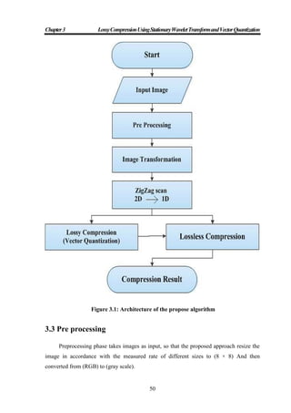
66. Chapter3 LossyCompressionUsingStationaryWaveletTransformandVectorQuantization
51
Resize image reduces in both horizontal and vertical direction using equation 3.1
fd (m, n) = f (2m,2n) ……………………..(1)
Where f (x, y) represents the original continuous image, fd (m, n) the sampled image.[71]
While gray scale ways to convert a full-color image to grayscale, equation 3.2, gray
scale algorithms utilizes the same basic three-step process:
1. Get the red, green, and blue values of a pixel
2. Use a fancy math to turn those numbers into a single gray value
3. Replace the original red, green, and blue values with the new gray value.
When describing grayscale algorithms, I‟m going to focus on step 2 – using math to
turn color values into a grayscale value. So, when you see a formula like this:
Gray = (Red + Green + Blue) / 3…………….(2)
Recognize that the actual code to implement such an algorithm looks like [71]:
6. Preprocessing Algorithm
RGB to Gray (image_matrix)
For Each Pixel in Image_matrix {
Red = Pixel. Red Green = Pixel. Green Blue = Pixel.Blue
Gray = (Red + Green + Blue) / 3
Pixel. Red = Gray
Pixel. Green = Gray
Pixel.Blue = Gray
}
Return image gray_matrix

67. Chapter3 LossyCompressionUsingStationaryWaveletTransformandVectorQuantization
52
Figure 3.2: Diagram conversion and downsizing
3.4 Image Transformation
Image transformation phase received the resizable gray scale images and produced
transformed images. This phase used the three types of wavelet transforms such as DWT,
LWT, and SWT.
3.4.1 Discrete Wavelet Transform
The Discrete Wavelet Transform (DWT) of image signals produces a nonredundant
image representation, which provides better spatial and spectral localization of image
formation, compared with other multi scale representations such as Gaussian and Laplacian
pyramid. Recently, Discrete Wavelet Transform has attracted more and more interest in
image fusion [17]. An image can be decomposed into a sequence of different spatial
resolution images using DWT. In case of a 2D image, an N level decomposition can be
performed, resulting in 3N+1 different frequency bands and it is shown in Figure. 3.3
Resizes to image
8x8
Image
2-D matrix (8x8)
Convert gray scale

68. Chapter3 LossyCompressionUsingStationaryWaveletTransformandVectorQuantization
53
Figure 3.3: 2D - Discrete wavelet transforms
3.4.2 Lifting Wavelet Transform
Lifting scheme algorithms have the advantage that they do not require temporary
arrays in the calculation steps, as is necessary for some versions of the Daubechies D4
Wavelet algorithm. The Predict step calculates the wavelet function in the wavelet
transform .This is a high Pass filter. The update step calculates the scaling function, which
results in a smoother version of the data [19].
This operation consists of three steps.
1) First, the input signal x[n] is down sampled into the even position signal xe (n)
and the odd position signal xo(n) , then modifying these values using
alternating prediction and updating steps.
xe (n) = x [2n] and xo(n) = x [2n+1]
2) A prediction step consists of predicting each odd sample as a linear
combination of the even samples and subtracting it from the odd sample to
form the prediction error.
3) An update step consists of updating the even samples by adding them to a
linear combination of the prediction error to form the updated sequence. The
prediction and update may be evaluated in several steps until the forward
transform is completed.

69. Chapter3 LossyCompressionUsingStationaryWaveletTransformandVectorQuantization
54
Figure 3.4: Diagram lifting wavelet scheme transform
3.4.3 Stationary Wavelet Transform
The Stationary wavelet transform (SWT) is a wavelet transform algorithm designed
to overcome the lack of translation-invariance of the discrete wavelet transforms (DWT).
Translation-invariance is achieved by removing the downsamplers and upsamplers in the
DWT and upsampling the filter coefficients by a factor of in the th level of the
algorithm. The SWT is an inherently redundant scheme as the output of each level of SWT
contains the same number of samples as the input – so for a decomposition of N levels
there is a redundancy of N in the wavelet coefficients[72].
The following block diagram depicts the digital implementation of SWT.
Figure 3.5 : 3 level Stationary wavelet transform filter bank
In the above diagram, filters in each level are up-sampled versions of the previous.
Figure 3.6: Stationary wavelet transforms filters

70. Chapter3 LossyCompressionUsingStationaryWaveletTransformandVectorQuantization
55
LLj+1(χ, γ) = L[n] L [m] LLj (2j+1 m- χ, 2j+1 n- γ)
LHj+1(χ, γ) = L[n] H [m] LLj (2j+1 m- χ, 2j+1 n- γ)
( 3 )
HLj+1(χ, γ) = H[n] L [m] LLj (2j+1 m- χ, 2j+1 n- γ)
HHj+1(χ, γ) = H[n] H [m] LLj (2j+1 m- χ, 2j+1 n- γ)
[MATLAB R2013a]

71. Chapter3 LossyCompressionUsingStationaryWaveletTransformandVectorQuantization
56
3.5 Zigzag Scan
Zigzag scans phase takes as an input the transformed images in 2D matrix and
produced images in 1D matrix, so that the frequency (horizontal + vertical) increases in
this order, and the coefficient variance decreases in this order [71].
Figure 3.7: Zigzag scan
3.6 Lossy Compression Vector quantization by Linde-Buzo-
Gray
Lossy compression technique provides a higher compression ratio than lossless
compression.
A lossy compression scheme, shown in Figure 3.8, may examine the color data for a
range of pixels, and identify subtle variations in pixel color values that are so minute that
the human eye/brain is unable to distinguish the difference between them.
Figure 3.8: Block diagram for lossy compression

72. Chapter3 LossyCompressionUsingStationaryWaveletTransformandVectorQuantization
57
Linde-Buzo-Gray (LBG) Algorithm They used a mapping function to partition
training vectors into N clusters. The mapping function is defined as:
Rk→CB
Let X = (x1, x2…xk) be a training vector and d(X; Y) be the Euclidean Distance
between any two vectors. The iteration of GLA for a codebook generation is given as
follows:
Step 1: Randomly generate an initial codebook CB0.
Step 2: i = 0.
Step 3: Perform the following process for each training vector.
Compute the Euclidean distances between the training vector and the
codewords in CBi. The Euclidean distance is defined as
d(X; C) = (√Σkt=1(xt− ct) 2) ........................................ (4)
Search the nearest codeword among CBi.
Step 4: Partition the codebook into N cells.
Step 5: Compute the centroid of each cell to obtain the new codebook CBi+1.
Step 6: Compute the average distortion for CBi+1. If it is changed by a small
enough amount since the last iteration, the codebook may converge and the
procedure stops. Otherwise, i = i + 1 and go to Step 3.

73. Chapter3 LossyCompressionUsingStationaryWaveletTransformandVectorQuantization
58
Figure 3.9: Flowchart of Linde Buzo Gray algorithm
LBG algorithm has the local optimization problem and the utility of each codeword
in the codebook is low. The local optimization problem means that the codebook
guarantees local minimum distortion, but not global minimum distortion
3.7 Lossless Compression
Lossless image compression schemes exploit redundancies without incurring any
loss of data. Lossless image compression is therefore exactly reversible. Lossless image
compression techniques first convert the images into the image pixels. Then processing is
done for each single pixel. Different Encoding Methods are, Huffman, Arithmetic.
In the lossless compression scheme, shown in Figure 3.10 the reconstructed image,
after compression, is numerically identical to the original image. It is used in many
applications such as ZIP file format & in UNIX tool gzip. It is important when the original
& the decompressed data be identical.

74. Chapter3 LossyCompressionUsingStationaryWaveletTransformandVectorQuantization
59
Figure 3.6: Block diagram for lossless compression
3.7.1 Arithmetic Coding
The main aim of Arithmetic coding is to assign an interval to each potential symbol.
Then a decimal number is assigned to this interval. The algorithm starts with an interval of
0.0 and 1.0. After each input symbol from the alphabet is read, the interval is subdivided
into a smaller interval in proportion to the input symbol‟s probability. This sub interval
then becomes the new interval and is divided into parts according to probability of symbols
from the input alphabet. This is repeated for each and every input symbol. And, at the end,
any floating point number from the final interval uniquely determines the input data.
Properties of Arithmetic Coding:
1- It uses binary fractional number.
2- Suitable for small alphabet with highly skewed probabilities.
3- Incremental transmission of bits are possible, avoiding working with higher and
higher precision numbers.
4- This encoding takes a stream of input symbol and it replaces it with floating
point numbers (0, 1).
5- It produces results in a stream of bits.

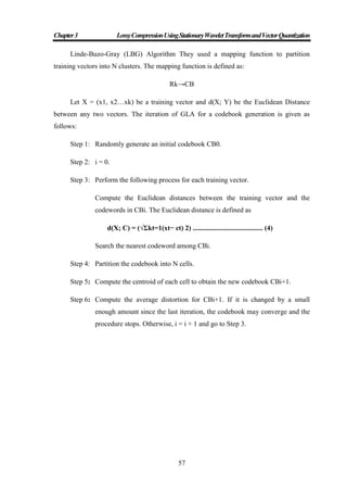
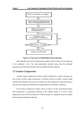
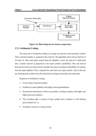
75. Chapter3 LossyCompressionUsingStationaryWaveletTransformandVectorQuantization
60
3.7.2 Huffman Coding
Uses Top-down approach The Huffman algorithm is simple and can be described in
terms of creating a Huffman code tree. The procedure for building this tree is:
1- Start with a list of free nodes, where each node corresponds to a symbol in the alphabet.
2- Select two free nodes with the lowest weight from the list.
3- Create a parent node for these two nodes selected and the weight is equal to the
weight of the sum of two child nodes.
4- Remove the two child nodes from the list and the parent node is added to the list of free
nodes.
5- Repeat the process starting from step-2 until only a single tree remains.
3.8 Compression Ratio
Compression Ratio: is the ratio of the size of the compressed database system with
the original size of the uncompressed database systems. Also known as compression,
power is a computer-science term used to quantify the reduction in data-representation size
produced by a data compression algorithm. Compression ratio is defined as follows: [1]
CR=
size of original image data
size of compressed image data
…………………(5)
3.9 Summary
In this chapter, we introduced our proposed approach called lossy image
compression using stationary wavelet transform and vector quantization, which consist of
four phases; namely: preprocessing, image transformation, zigzag scan, and lossy/lossless
compression. In preprocessing phase, we take an image as inputs and produced gray scale
resizable images. In image transformation phase, we take the result of preprocessing phase
and applied transformation techniques such as SWT to transformed our images, so in
zigzag scan phase, we mapping our images from two dimension matrix into one dimension
matrix. Finally, in the Lossy/Lossless phase, we applied vector quantization and other
techniques to compress our images in a sufficient way.

76. Chapter 4 Experiments & Results Analysis
61
EXPERIMENTS AND RESULTS ANALYSIS
This chapter reports selected results from the experimental evaluation, including
several experimental results performed to ascertain and assess the accuracy and
robustness of the approach that proposed in chapter 3 as follows
4.1 Data set and its Characteristics
Used in the proposed system 5 images (2 gray scale, 3 RBG)
1 - Lena.jpg, gray scale, Dimensions 512*512, Size 37.7 KB.
2 - Cameraman.jpg, gray scale, Dimensions 256*256, Size 40 KB.
3 - Tulips.jpg, RBG, Dimensions 1024*768, Size 606 KB.
4 - White flower.png, RBG, Dimensions 497*498, Size 198 KB.
5 - Fruits.png, RBG, Dimensions 512*512, Size 461 KB.
Work experiment in Matlab R2013a.
4.2 Image formats used:
Lena.jpg Cameraman.jpg

77. Chapter 4 Experiments & Results Analysis
62
Tulips.jpg White flower.png
Fruits.png
4.3 PC Machine
Machine name: OMAR-PC
Operating System: Windows 7 Ultimate 32-bit
System Model: HP 15 Notebook PC
BIOS: InsydeH2O Version 03.73.06F.31
Processor: Intel(R) Core(TM) i5-4210U CPU @ 1.70GHz (4 CPUs), ~2.4GHz
Memory: 4096 MB RAM
Hard Disk: 500 GB
Card name: Intel(R) HD Graphics Family
Display Memory: 1189 MB

78. Chapter 4 Experiments & Results Analysis
63
4.4 Experiments
In this section of the performance of three types of wavelet transform (SWT, DWT,
and LWT) and the impact of each type on the image lossy compression performance also it
shows the lossy using vector quantization (LBG) and lossless compression using
Arithmetic coding and Huffman coding.
4.4.1 Experiment (1)
In this experiment, four operations:
1- DWT-Zigzag-Arithmetic
2- DWT-Zigzag-LBG–Arithmetic
3- DWT-Zigzag-Huffman
4- DWT-Zigzag-LBG–Huffman
Table 4.1 showing results for the process lossy and lossless image compression of
the five images using the discrete wavelet transform with arithmetic coding and Huffman
coding without the use of the LBG, as well as with the use of the LBG and that using three
decomposition levels.

79. Chapter 4 Experiments & Results Analysis
64
Table 4.1: Discrete wavelet transforms, vector quantization (LBG), Arithmetic
and Huffman coding
DWT
DWT Zigzag
Arithmetic
DWT Zigzag LBG &
Arithmetic
DWT Zigzag
Huffman
DWT Zigzag LBG &
Huffman
Image Level C.Ratio
Running
time(Sec)
C.Ratio psnr
Running
time(Sec)
C.Ratio
Running
time(Sec)
C.Ratio psnr
Running
time(Sec)
Lena
1 1.1934 0.4919 1.2549 18.2975 0.0157 1.1403 0.0735 1.1879 18.2975 0.057
2 1.261 0.0459 1.3027 18.2745 0.012 1.0556 0.0785 1.1403 18.2745 0.0438
3 1.2994 0.0721 1.28 18.2449 0.0164 1.026 0.1237 1.1583 18.2449 0.0465
Camera
man
1 1.2518 0.0351 1.2549 18.2588 0.0158 1.177 0.0611 1.2549 18.2588 0.0421
2 1.2549 0.0498 1.2641 18.1648 0.0125 1.1557 0.0904 1.2047 18.1648 0.0459
3 1.2896 0.062 1.2457 18.0733 0.0111 1.1454 0.1148 1.2018 18.0733 0.0609
Tulips
1 1.1851 0.093 1.2427 17.4091 0.0153 1.1824 0.1483 1.199 17.4091 0.0657
2 1.1934 0.0965 1.28 17.4196 0.0105 1.177 0.1231 1.199 17.4196 0.0458
3 1.0916 0.1131 1.2864 17.3919 0.011 1.1479 0.2548 1.1824 17.3919 0.0447
White
flower
1 1.0622 0.0431 1.2549 16.7503 0.0128 1.0385 0.0764 1.1879 16.7503 0.0413
2 1.1203 0.0546 1.2549 16.7639 0.0106 1.0893 0.075 1.1934 16.7639 0.0458
3 1.0916 0.0457 1.2518 16.8377 0.0169 1.026 0.0785 1.1879 16.8377 0.047
Fruits
1 1.2047 0.0489 1.28 17.5693 0.013 1.1428 0.0829 1.2104 17.5693 0.0513
2 1.2104 0.0922 1.2427 17.6137 0.0139 1.1302 0.0967 1.2161 17.6137 0.044
3 1.2161 0.0508 1.2641 17.5718 0.0148 1.1252 0.0831 1.1962 17.5718 0.0455
In level - 1, we find that DWT Zigzag LBG & Arithmetic the best thing, In terms of
compression ratio and compression time. And find that Arithmetic the best of Huffman
with everyone.
In level - 2, we find that DWT & LBG Zigzag Arithmetic the best thing, In terms of
compression ratio and compression time and find that Arithmetic the best of Huffman with
everyone, and high rate compression ratio in level 2 more level 1.
In level - 3, we find that DWT & LBG Zigzag Arithmetic the best thing, In terms of
compression ratio and compression time and find that Arithmetic the best of Huffman with
everyone, low rate compression ratio in level 3 for level 1 and level 2.

80. Chapter 4 Experiments & Results Analysis
65
4.4.2 Experiment (2)
In this experiment, four operations:
1- LWT-Zigzag-Arithmetic
2- LWT-Zigzag-LBG–Arithmetic
3- LWT-Zigzag- Huffman
4- LWT-Zigzag-LBG–Huffman
Table 4.2 shows the results for the process lossy and lossless image compression of
the five images using the lifting wavelet transform with arithmetic coding and Huffman
coding without the use of the LBG, as well as with the use of the LBG and that using three
decomposition levels.

81. Chapter 4 Experiments & Results Analysis
66
Table 4.2: Lifting wavelet transforms, vector quantization (LBG), Arithmetic and
Huffman coding
LWT
LWT Zigzag
Arithmetic
LWT Zigzag LBG &
Arithmetic
LWT Zigzag
Huffman
LWT Zigzag LBG &
Huffman
Image Level C.Ratio
Runningtime
(Sec)
C.Ratio psnr
Runningtime
(Sec)
C.Ratio
Running
time(Sec)
C.Ratio psnr
Running
time(Sec)
Lena
1 1.4065 0.3177 1.6842 13.1876 0.0081 1.3763 0.0674 1.4545 13.1876 0.0216
2 1.3763 0.4231 1.641 11.9784 0.0097 1.113 0.0527 1.4712 11.9784 0.0162
3 1.1636 0.0489 1.6842 17.4394 0.0073 1.094 0.0708 1.4545 17.4394 0.0154
Camera
man
1 1.5421 0.0658 1.641 13.6895 0.0076 1.2673 0.0511 1.4712 13.6895 0.017
2 1.2427 0.0326 1.7534 12.7065 0.0093 1.1327 0.0401 1.4222 12.7065 0.0155
3 1.1428 0.0376 1.6623 16.9649 0.0074 1.1228 0.0836 1.4222 16.9649 0.0204
Tulips
1 1.0275 0.0947 1.7777 16.2979 0.0122 1.3763 0.1357 1.4545 17.0032 0.0196
2 1.4382 0.1336 1.641 12.2671 0.0111 1.094 0.1054 1.4712 12.2671 0.0225
3 1.2549 0.1174 1.6842 19.5465 0.0073 1.0578 0.1067 1.4545 19.5465 0.0162
White
flower
1 1.3913 0.04 1.641 15.4661 0.0073 1.3763 0.0537 1.4712 15.4661 0.0182
2 1.3061 0.0473 1.7066 14.3703 0.0118 1.2549 0.0528 1.4545 14.3703 0.0186
3 1.1636 0.0827 1.641 16.1241 0.0074 1.2549 0.0599 1.4712 16.1241 0.0162
Fruits
1 1.2397 0.0453 1.7777 12.3394 0.0091 1.1228 0.0557 1.4065 12.3394 0.016
2 1.3763 0.079 1.641 12.2289 0.0089 1.113 0.0902 1.4712 12.2289 0.0164
3 1.1962 0.0874 1.6202 18.1602 0.0074 1.0756 0.0652 1.4065 18.1602 0.0164
In level - 1, we find that LWT Zigzag LBG & Arithmetic the best thing, In terms of
compression ratio and compression time. And find that arithmetic the best of huffman with
everyone.
In level - 2, we find that LWT & LBG Zigzag Arithmetic the best thing, In terms of
compression ratio and compression time and find that Arithmetic the best of Huffman with
everyone, and low rate compression ratio in level 2 for level 1.
In level - 3, we find that LWT & LBG Zigzag Arithmetic the best thing, In terms of
compression ratio and compression time and find that Arithmetic the best of Huffman with
everyone, low rate compression ratio in level 3 for level 1 and level 2.

82. Chapter 4 Experiments & Results Analysis
67
4.4.3 Experiment (3)
In this experiment, four operations:
1- SWT-Zigzag-Arithmetic
2- SWT–Zigzag-LBG–Arithmetic
3- SWT-Zigzag- Huffman
4- SWT–Zigzag-LBG–Huffman
In the table 4.3, shows the results for the process lossy and lossless image
compression of five images using stationary wavelet transform with arithmetic coding and
Huffman coding without the use of the LBG, as well as with the use of the LBG and that
using three decomposition levels.

83. Chapter 4 Experiments & Results Analysis
68
Table 4.3: Stationary wavelet transforms, vector quantization (LBG), Arithmetic
and Huffman coding
SWT
SWT Zigzag
Arithmetic
SWT Zigzag LBG &
Arithmetic
SWT Zigzag
Huffman
SWT Zigzag LBG &
Huffman
Image Level C.Ratio
Running
time(Sec)
C.Ratio psnr
Running
time(Sec)
C.Ratio
Running
time(Sec)
C.Ratio psnr
Running
time(Sec)
Lena
1 4.3667 0.1155 5.0073 18.0121 0.0685 2.6256 0.859 4.8188 18.0121 0.0473
2 4.3667 0.0414 5.0073 18.8982 0.012 2.6256 0.8439 4.8188 18.8982 0.0455
3 4.3667 0.1906 5.0073 18.8982 0.0137 2.6256 0.8576 4.8188 18.8982 0.0422
Camera
man
1 4.1042 0.0651 5.0073 16.8483 0.011 2.6771 0.9157 4.853 16.8483 0.0419
2 4.1042 0.0537 5.0073 18.1099 0.011 2.6771 0.8346 4.853 18.1099 0.0447
3 4.1042 0.0398 5.0073 18.1099 0.0103 2.6771 0.9481 4.853 18.1099 0.0462
Tulips
1 3.8641 0.0934 5.6574 18.6787 0.0099 2.7563 0.8965 4.6022 18.6787 0.0461
2 3.8641 0.0961 5.6574 17.1798 0.0116 2.7563 0.9289 4.6022 17.1798 0.0456
3 3.8641 0.0969 5.6574 17.1798 0.0121 2.7563 0.8919 4.6022 17.1798 0.0421
White
flower
1 3.7372 0.0393 4.9588 17.3002 0.0117 2.7018 0.8483 4.6757 17.3002 0.0459
2 3.7372 0.0392 4.9588 17.2142 0.0128 2.7018 0.8438 4.6757 17.2142 0.0459
3 3.7372 0.041 4.9588 17.2142 0.012 2.7018 0.8411 4.6757 17.2142 0.0412
Fruits
1 3.828 0.0584 5.1072 18.9503 0.0132 2.7379 0.8438 4.3206 18.9503 0.0435
2 3.828 0.458 5.1072 18.1739 0.0105 2.7379 0.8585 4.3206 18.1739 0.0567
3 3.828 0.1188 5.1072 18.1739 0.012 2.7379 0.8463 4.3206 18.1739 0.043
In level - 1, we find that SWT Zigzag LBG & Arithmetic the best thing, In terms of
compression ratio and compression time. And find that Arithmetic the best of Huffman
with everyone.
In level - 2 , we find that SWT & LBG Zigzag Arithmetic the best thing, In terms of
compression ratio and compression time and find that Arithmetic the best of Huffman with
everyone , and firming (SWT) as in level 1 in compression ratio .
In level - 3, we find that SWT & LBG Zigzag Arithmetic the best thing, In terms of
compression ratio and compression time and find that Arithmetic the best of Huffman with
everyone, and firming (SWT) as in level 1 & 2.

84. Chapter 4 Experiments & Results Analysis
69
4.4.4 Average Compression Ratio
Level – 1
Figure 4.1: Chart shows the result average compression ratio in level – 1
In level - 1, we find that SWT & LBG Zigzag arithmetic the best thing, and find that
arithmetic the best of Huffman with everyone.
0.5
1
1.5
2
2.5
3
3.5
4
4.5
5
5.5
Arithmatic LBG Zigzag
Arithmatic
Huffman LBG Zigzag Huffman
Average Compression Ratio (C.R) in Level -1
SWT
DWT
LWT

85. Chapter 4 Experiments & Results Analysis
70
Level – 2
Figure 4.2: Chart shows the result average compression ratio in level - 2
In level - 2 , We find that SWT & LBG Zigzag Arithmetic the best thing , and find
that Arithmetic the best of Huffman with everyone, and firming (SWT) as in level 1, and
the high rate of (DWT) and low rate (LWT) .
Level – 3
Figure 4.3: Chart shows the result average compression ratio in level – 3
0.5
1
1.5
2
2.5
3
3.5
4
4.5
5
5.5
Arithmatic LBG Zigzag
Arithmatic
Huffman LBG Zigzag Huffman
Average Compression Ratio (C.R) in Level - 2
SWT
DWT
LWT
0.5
1
1.5
2
2.5
3
3.5
4
4.5
5
5.5
Arithmatic LBG Zigzag
Arithmatic
Huffman LBG Zigzag
Huffman
Average Compression Ratio (C.R) in Level - 3
SWT
DWT
LWT

86. Chapter 4 Experiments & Results Analysis
71
In level - 3, we find that SWT & LBG Zigzag Arithmetic the best thing, and find that
Arithmetic the best of Huffman with everyone, and firming (SWT) as in level 1 & 2, and
the low rate of (DWT) and low rate (LWT).
4.5 Results Analysis
1- Compression ratio in LBG Bigger without LBG.
2- Stationary wavelet transforms best transform.
3- Arithmetic coding best of Huffman coding.
4- That's the best path for image compression is Stationary wavelet transform -
zigzag scans – Vector Quantization (LBG) - Arithmetic coding where the
compression ratio achieved 5.1476 in 0.02286 Running time (Sec).
Figure 4.4: Best path for lossy image compression
Image SWT
Zigzag
scan
Vector
Quantization
(LBG)
Arithmetic
coding
Pre-
processin
g

87. Chapter 5 Conclusion & Future Work
72
CONCLUSION AND FUTURE WORK
5.1 Conclusion
This thesis introduced a new approach that is built to work on image compression.
Our approach used vector quantization LBG, Arithmetic coding and Huffman coding with
three types of wavelet transforms such as Discrete Wavelet Transform DWT, Lifting
Wavelet Transform LWT, and Stationary Wavelet Transform SWT on three decomposition
levels. As in Stationary Wavelet Transform (SWT) compression ratio is fixed at a high
level, and Discrete Wavelet Transform (DWT) compression ratio variable at a high level,
either Lifting Wavelet Transform (LWT) is less than the compression at high level. We
conclude that arithmetic coding is better than Huffman coding in terms of compression
ratio and time. We found that the best way to compression in this system is the stationary
wavelet transforms (SWT), LBG vector quantization, and arithmetic coding where it gives
the best compression ratio with less time possible. Also the size of compressed data by
adding arithmetic coding is better than adding Huffman coding to SWT.

88. Chapter 5 Conclusion & Future Work
73
5.2 Future Work
Lossy image compression process is important to achieve high compression ratios.
1- It will be possible in the future to achieve these goals through the addition of fuzzy
logic to wavelet transform techniques.
2- It will be possible in the future to achieve these goals through using the new
families of the wavelet transforms such as chirplet transform or other
transformation techniques.
3- Important issues are security sends compressed images can be achieved to using
several methods in order to protect the transmissions of images. The protection of
visual data can be done by using encryption or watermarking algorithms or by
combining these two approaches.

89. References
74
REFERENCES
1. Kodituwakku SR, Amarasinghe U.S. Comparison of lossless data compression
algorithms for text data. Indian J Comput Sci Eng 2010; 1(4): 416-25
2. Melwin S, Solomon AS, Nachappa MN. A survey of compression techniques. Int J
Recent Technol Eng 2013; 2(1): 152-6.
3. Gupta P, Purohit GN, Bansal V. A survey on image compression techniques. Int J
Adv Res Comput Commun Eng 2014; 3(8): 7762-8.
4. Kaur M, Kaur G. A survey of lossless and lossy image compression techniques. Int J
Adv Res Comput Sci Software Eng 2013; 3(2): 323-6.
5. Nashat S, Abdullah A, Abdullah MZ. A stationary wavelet edge detection algorithm
for noisy images. Tech Rep School Electr Electron Eng 2011; 1:1-9.
6. Siva Kumar B, Nagaraj S. Discrete and stationary wavelet decomposition for
IMAGE resolution enhancement. IJETT 2013; 4(7): 2885-9.
7. Sathappan S. A vector quantization technique for image compression using modified
fuzzy possibilistic C-means with weighted mahalanobis distance. Int J Innovative
Res Comput Commun Eng 2013; 1(1): 12-20.
8. Huan CJ, Yeh CY, Hwang SH. An improvement of the triangular inequality elimination
algorithm for vector quantization. Appl Math Inf Sci 2015; 9: 229-35.
9. Samra HS. Image compression techniques. Int J Comput Technol 2012; 2(2): 49-52.
10. Mittal M, Lamba R. Image compression using vector quantization algorithms: a
review. Int J Adv Res Comput Sci Software Eng 2013; 3(6): 354-8.
11. Vlajic N, Card HC. Vector quantization of images using modified adaptive
resonance algorithm for hierarchical clustering. IEEE Neural Netw Trans 2001;
12(5): 1147-62.
12. Amin B, Amrutbhai P. Vector quantization based lossy image compression using
wavelets – a review. Int J Innovative Res Sci Eng Technol 2014; 3(3): 10517- 23.

90. References
75
13. Chowdhury MMH, Khatun A. Image compression using discrete wavelet transform.
Int J Comput Sci Issues 2012; 9(4): 327-30.
14. Kannan K, Perumal AS, Arulmozhi K. Optimal decomposition level of discrete,
stationary and dual tree complex wavelet transform for pixel based fusion of multi-
focused images. Serbian J Elect Eng 2010; 7(1): 81-93.
15. Kaur P, Lalit G. Comparative analysis of DCT, DWT &LWT for image
compression. Int J Innovative Technol Explor Eng 2012; 1(3): 2278-3075.
16. Majumder S, Meitei NL, Singh AD, Mishra M. Image compression using lifting
wavelet transform. Int Conf Adv Commun Netw Comput 2010; 2010: 10-3.
17. Bhavani S, Thanushkodi K. A survey on coding algorithms in medical image
compression. Int J Comput Sci Eng 2010; 2(5): 1429-34.
18. Bonifati A, Lorusso M, Sileo D. XML lossy text compression: a preliminary study.
In: Bellahsene Z (ed). XSym 2009. Berlin, Germany: Springer-Verlag Berlin
Heidelberg; 2009. p.113.
19. Graps A. An introduction to wavelets. IEEE Computat Sci Eng 1995; 2(2): 50-61.
20. Lin PL. An introduction to wavelet transform. Tech Rep Graduate Inst Commun
Eng Nat 2007; 1: 1-24.
21. Roy S, Sen AK, Sinha N. VQ-DCT based image compression: a new hybrid
approach. Assam Univ J Sci Technol 2010; 5(2): 73-80.
22. Taubman DS, Marcellin MW. JPEG2000: Image compression fundamentals,
standards, and practice. New York: Springer Science+Business Media; 2002. p.780.
23. Chanda B, Majumder DD. Digital image processing and analysis. India: PHI
Learning Pvt Ltd; 2004.p.384.
24. Gonzalez R, Richard RC. Digital image processing. 3rd
ed. New Jersey: Pearson
Education; 2002.p.103.

91. References
76
25. Kashyap N, Singh SN. Review of image compression and comparison of its
algorithms. Int J Inf Sci Comput 2014; 1(1): 49-55.
26. Vimala S, Usha Rani P, Anitha Joseph J. A hybrid approach to compress still images
using wavelets and vector quantization. Int J Eng Adv Technol 2015; 4(4): 56-0.
27. Lees K. Image compression using wavelets. Master Thesis. , Virgina Polytechnic
Institute and State University, Virgina; 2002.
28. Pal AK, Sar A. An efficient codebook initialization approach for LBG algorithm. Int
J Comput Sci Eng Appl 2011; 1(4): 72-80.
29. Lu TC, Chang CY. A survey of VQ codebook generation. J Inf Hiding Multimedia
Signal Proc 2010; 1(3): 190-203.
30. Al-Allaf ONA. Codebook enhancement in vector quantization image compression
using back propagation neural network. J Appl Sci 2011; 11: 3152-60.
31. Panda SS, Prasad MSRS, Prasad MNM, Naidu CS. Image compression using back
propagation neural network. Int J Eng Sci Adv Technol 2012; 2: 74-8.
32. Al-Allaf ONA. Fast back propagation neural network algorithm for reducing
convergence time of BPNN image compression. Proceedings of the 5th
International
Conference on IT & Multimedia at UNITEN, Malaysia; 2011. pp. 1-6.
33. Al-Allaf ONA. Improving the performance of back propagation neural network
algorithm for image compression/decompression system. J Comput Sci 2010; 6(11):
1347-54.
34. Maan AJ. Analysis and comparison of algorithms for lossless data compression. Int
J Inf Computat Technol 2013;3(3):139-46.
35. Vijayvargiya G, Silakari S, Pandey R. A survey: various techniques of image
compression. IJCSIS 2013; 11(10): 1-5.
36. Huang JY, Liang YC, Huang YM. Secure integer arithmetic coding with adjustable
interval size. Proceedings of 19th
Asia-Pacific Conference on Communications
(APCC), Bali, Indonesia; 2013. pp. 683-7.

92. References
77
37. Jindal V, Verma AK, Bawa S. Impact of compression algorithms on data
transmission. Int J Adv Comput Theory Eng 2013; 2(2):2319-526.
38. Iombo C. Predictive data compression using adaptive arithmetic coding. PhD
Thesis. Agricultural and Mechanical College, Louisiana State University; 2007.
39. Wiegand T, Sullivan G, Bjontegaard G, Luthra A. Overview of the H.264/AVC
video coding standard. IEEE Trans Circuits Syst Video Technol 2003; 13(7): 560–
76.
40. Kim H, Villasenor J, Wen J. Secure arithmetic coding using interval splitting.
Proceedings of the Thirty-Ninth Asilomar Conference on Signals, Systems and
Computers; Oct. 28 – Nov. 1, 2005. pp. 1218–21.
41. Wen JT, Kim H, Villasenor JD. Binary arithmetic coding with key-based interval
splitting. IEEE Signal Proc Lett 2006;13: 69–72.
42. Jakimoski G, Subbalakshmi KP. Cryptanalysis of some multimedia encryption
schemes. IEEE Trans Multimedia 2008; 10(3): 330–8.
43. Katti RS, Srinivasan SK, Vosoughi A. On the security of key-based interval splitting
arithmetic coding with respect to message Indistinguishability. IEEE Trans Inf
Forensics Sec 2012; 7(3): 895-903.
44. Kim H, Wen JT, Villasenor JD. Secure arithmetic coding. IEEE Trans Signal Proc
2007; 55: 2263–72.
45. Zhou J, Au OC, Wong PHW. Adaptive chosen-ciphertext attack on secure
arithmetic coding. IEEE Trans Signal Proc 2009; 57(5): 1825–38.
46. Sun HM, Wang KH, Ting WC. On the security of secure arithmetic code. IEEE
Trans Inf Forensics Sec 2009; 4(4): 781-9.
47. Grangetto M, Magli E, Olmo G. Multimedia selective encryption by means of
randomized arithmetic coding. IEEE Trans Multimedia 2006; 8(5): 905–17.

93. References
78
48. Katti RS, Srinivasan SK, Vosoughi A. On the security of randomized arithmetic
codes against ciphertext-only attacks. IEEE Trans Inf Forensics Sec 2011; 6(1): 19–
27.
49. Huang YM, Liang YC. Secure arithmetic coding algorithm based on integer
implementation. Proceedings of the 11th
IEEE International Symposium on
Communications and Information Technologies, Hangzhou, China, Oct. 12-14,
2011. pp. 518-21.
50. Navneet G, Kaur AP. Review: analysis and comparison of various techniques of
image compression for enhancing the image quality. J Basic Appl Eng Res 2014;
1(7): 5-8.
51. Porwal S, Chaudhary Y, Joshi J, Jain M. Data compression methodologies for
lossless data and comparison between algorithms. I J Eng Sci Innovative Technol
2013; 2(2): 142-7.
52. Hasan R. Data compression using huffman based LZW encoding technique. Int J Sci
Eng Res 2011; 2(11): 1-7.
53. Shen JJ, Huang HC. An adaptive image compression method based on vector
quantization. Proceeding of the International Conference on Pervasive Computing,
Signal Processing and Applications, 17-19 Sept, 2010. Harbin; 2010. pp. 377-81.
54. Yerva S, Nair S, Kutty K. Lossless image compression based on data folding.
Proceeding of the IEEE-International Conference on Recent Trends in Information
Technology, ICRTIT 2011, Anna University, June 3-5, 2011, IEEE, Chennai; 2011.
pp. 999-1004.
55. Jassim FA, Qassim HE. Five modulus method for image compression. SIPIJ 2012;
3(5): 19-28.
56. Dwivedi A, Bose NS, Kumar A, Kandula P, Mishra D, Kalra PK. A novel hybrid
image compression technique. Proceedings of the ASID 6, 8-12 Oct, 2012, New
Delhi; 2012. pp. 492-5.

94. References
79
57. Tan YF, Tan WN. Image compression technique utilizing reference points coding
with threshold values. Proceedings of the Audio, Language and Image Processing
(ICALIP), 2012 International Conference on 16-18 July 2012 , Shanghai; 2012. pp.
74-7.
58. Sahami S, and Shayesteh MG. Bi-level image compression technique using neural
networks. IET Image Process 2012; 6(5): 496–506.
59. Rengarajaswamy C, Rosaline SI. SPIHT compression of encrypted images.
Proceedings of 2013 IEEE Conference on Information and Communication
Technologies, Shanghai; 2013. pp. 336-41.
60. Srikanth S, Meher S. Compression efficiency for combining different embedded
image compression techniques with Huffman encoding. Proceeding of International
conference on Communication and Signal Processing, April 3-5, 2013, India; 2013.
pp. 816-20.
61. Shantagiri PV, Saravanan KN. Pixel size reduction lossless image compression
algorithm. Int J Comput Sci Inf Technol 2013; 5: 97-5.
62. Rajakumar K, Arivoli T. Implementation of multiwavelet transform coding for
lossless image compression. Proceeding of the Information Communication and
Embedded Systems (ICICES), 2013 International Conference on 21-22 Feb. 2013 .
Chennai; 2013. pp. 634-7.
63. Dharanidharan S, Manoojkumaar SB, Senthilkumar D. Modified international data
encryption algorithm using in image compression techniques. Int J Eng Sci
Innovative Technol 2013; 2(2): 186-91.
64. Chowdhury MMH, Khatun A. Image compression using discrete wavelet transform.
Int J Comput Sci Issues 2012; 9(4): 327-30.
65. Patel TS, Modi R, Patel KJ. Image compression using DWT and vector quantization.
Int J Innovative Res Comput Commun Eng 2013; 1(3): 651-9.

95. References
80
66. Yamanaka O, Yamaguchi T, Maeda J, Suzuki Y. Image compression using wavelet
transform and vector quantization with variable block size. In: Proceeding of the
2008 IEEE Conference on Soft Computing in Industrial Applications (SMCia/08),
June 25-27, 2008, Muroran, JAPAN; 2008. pp. 359-64.
67. Shanmugasundaram S, Lourdusamy R. A comparative study of text compression
algorithms. Int J Wisdom Based Comput 2011; 1(3): 68-76.
68. Kumar J, Kumar M. Lossless fractal image compression mechanism by applying
exact self-similarities at same scale. In: Das VV, Thankachan N (eds). CIIT 2011,
CCIS 250. Berlin, Germany: Springer-Verlag Berlin Heidelberg; 2011. pp. 584–9
69. Samet A, Ben Ayed MA, Loulou MS, Masmoudi N, Kamoun L. JPEG 2000:
performance and evaluation. Proceeding In Systems, Man and Cybernetics, 2002
IEEE International Conference. Kowloon;2002. p.6.
70. Garg R, Gulshan V. JPEG image compression. Lecture Note, Dec, 2005. Available
from: rahuldotgarg.appspot.com/data/JPEG.pdf.
71. Blelloch GE. Introduction to data compression. Computer Science Department,
Carnegie Mellon University, Mellon; 2013. pp.1-55.
72. Nema M, Gupta L, Trivedi NR. Video compression using SPIHT and SWT wavelet.
Int J Electron Commun Eng 2012; 5(1): 1-8.

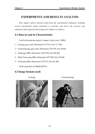
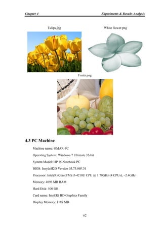
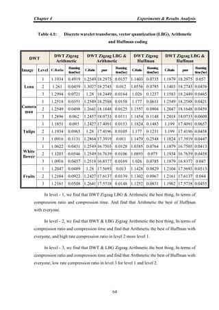
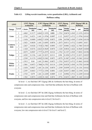
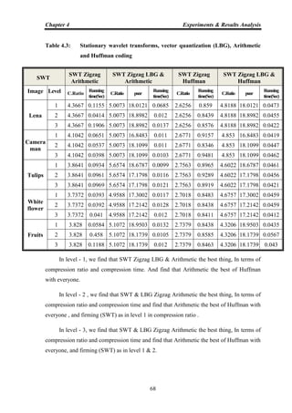
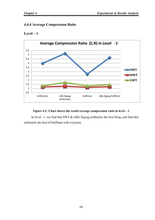
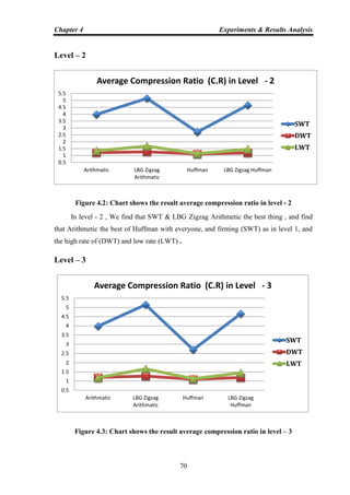
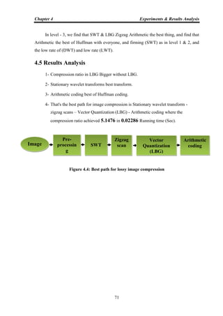
96. Appendix (I) Programs Appendices
1
APPENDIX (I)
Implementation of Lossy Compression Using Stationary
Wavelet Transform and Vector Quantization
1- Stationary Wavelet Transform (SWT)
1.1. Swt_Zigzag_Arithmetic
function [out] = swt_Zigzag_Arithmetic(Level,SX,SY)
% clc; % Clear the command window.
% close all; % Close all figures (except those of imtool.)
% imtool close all; % Close all imtool figures if you have the Image Processing Toolbox.
% clear; % Erase all existing variables. Or clearvars if you want.
% workspace; % Make sure the workspace panel is showing.
Setdemorandstream(96868483);
disp('Running ..');
SX=str2num(get(SX,'String'));
SY=str2num(get(SY,'String'));
Level=str2num(get(Level,'String'));
[filename, pathname]=uigetfile({'*.jpg';'*.bmp';'*.png'},'Select an image');
tic;
dbstop if error
ab=strcat(pathname,filename);
gmap = [0:255;0:255;0:255]'/255;
X = imread(ab);
X = imresize(X, [SX SY]);
[ORX,ORY]=size(X);
[X,map] = rgb2ind(X,gmap);
I=double(X);
[xx,yy]=size(I);
% Image coding.
Nbcol = size(map,1);
cod_X = wcodemat(I,nbcol);
%=========================SWT============================

97. Appendix (I) Programs Appendices
2
[ca,chd,cvd,cdd] = swt2(X,Level,'db1');
cod_ca = wcodemat(ca(:,:,1),nbcol);
cod_chd = wcodemat(chd(:,:,1),nbcol);
cod_cvd = wcodemat(cvd(:,:,1),nbcol);
cod_cdd = wcodemat(cdd(:,:,1),nbcol);
decl = [cod_ca,cod_chd;cod_cvd,cod_cdd];
imwrite(cod_ca,map,'myclown.png')
Xswt = imread('myclown.png');
% figure;imshow(Xswt)
%=========================Zigzag============================
p=zigzag (Xswt);
%=======================Arithmatic===========================
pp=p';
BB = sort(pp);
BB= unique(BB);
[M N]=size(pp);
ppnew=zeros(M,1);
for k=1:M
ppnew(k,1) =find(BB==pp(k,1));
end
[M N]=size(ppnew');
v=max(ppnew);
counts = [1:1:v*2]; % Distinct data symbols appearing in sig
code = arithenco(ppnew',counts);
CompressionRatio = CR(decl,code)
toc;
1.2. Swt_LBGVQ_Zigzag_Arithmetic
function [out] = SWT_LBGVQ_Zigzag_Arithmetic(Level,SX,SY)
% clc; % Clear the command window.
% close all; % Close all figures (except those of imtool.)
% imtool close all; % Close all imtool figures if you have the Image Processing Toolbox.
% clear; % Erase all existing variables. Or clearvars if you want.

98. Appendix (I) Programs Appendices
3
% workspace; % Make sure the workspace panel is showing.
setdemorandstream(96868483);
disp('Running ..');
SX=str2num(get(SX,'String'));
SY=str2num(get(SY,'String'));
Level=str2num(get(Level,'String'));
[filename, pathname]=uigetfile({'*.jpg';'*.bmp';'*.png'},'Select an image');
load parameter;
global para;
tic;
ab=strcat(pathname,filename);
gmap = [0:255;0:255;0:255]'/255;
X = imread(ab);
X = imresize(X, [SX SY]);
[ORX,ORY]=size(X);
[X,map] = rgb2ind(X,gmap);
I=double(X);
[xx,yy]=size(I);
% Image coding.
nbcol = size(map,1);
cod_X = wcodemat(I,nbcol);
% subplot(333)
% image(cod_X)
% title('Original image');
% colormap(map)
%=========================SWT============================
[ca,chd,cvd,cdd] = swt2(X,Level,'db1');
cod_ca = wcodemat(ca(:,:,1),nbcol);
cod_chd = wcodemat(chd(:,:,1),nbcol);
cod_cvd = wcodemat(cvd(:,:,1),nbcol);
cod_cdd = wcodemat(cdd(:,:,1),nbcol);
decl = [cod_ca,cod_chd;cod_cvd,cod_cdd];

99. Appendix (I) Programs Appendices
4
imwrite(cod_ca,map,'myclown.png')
x = imread('myclown.png');
% figure;imshow(Xswt)
%=========================Vector Quantization==================
original=x;
[v]=trainlvq(x,0);
compressed=v;
[y]=testlvq1(x);
[psnrvalue]=psnr2(original,y,255)
%=========================Zigzag============================
p=zigzag (Xswt);
%=======================Arithmatic===========================
pp=p';
BB = sort(pp);
BB= unique(BB);
[M N]=size(pp);
ppnew=zeros(M,1);
for k=1:M
ppnew(k,1) =find(BB==pp(k,1));
end
[M N]=size(ppnew');
v=max(ppnew);
counts = [1:1:v]; % Distinct data symbols appearing in sig
code = arithenco(ppnew',counts);
CompressionRatio = CR(decl,code)
toc;
1.3. Swt_Zigzag_Huffman
function [out] = swt2_Zigzag_Hufman(Level,SX,SY)
% clc; % Clear the command window.
% close all; % Close all figures (except those of imtool.)
% imtool close all; % Close all imtool figures if you have the Image Processing Toolbox.
% clear; % Erase all existing variables. Or clearvars if you want.

100. Appendix (I) Programs Appendices
5
% workspace; % Make sure the workspace panel is showing.
setdemorandstream(96868483);
disp('Running ..');
% set(0, 'RecursionLimit', 100000)
SX=str2num(get(SX,'String'));
SY=str2num(get(SY,'String'));
Level=str2num(get(Level,'String'));
[filename, pathname]=uigetfile({'*.jpg';'*.bmp';'*.png'},'Select an image');
tic;
dbstop if error
ab=strcat(pathname,filename);
gmap = [0:255;0:255;0:255]'/255;
X = imread(ab);
X = imresize(X, [SX SY]);
[ORX,ORY]=size(X);
[X,map] = rgb2ind(X,gmap);
I=double(X);
[xx,yy]=size(I);
% Image coding.
nbcol = size(map,1);
cod_X = wcodemat(I,nbcol);
%============================SWT===========================
[ca,chd,cvd,cdd] = swt2(X,Level,'db1');
cod_ca = wcodemat(ca(:,:,1),nbcol);
cod_chd = wcodemat(chd(:,:,1),nbcol);
cod_cvd = wcodemat(cvd(:,:,1),nbcol);
cod_cdd = wcodemat(cdd(:,:,1),nbcol);
decl = [cod_ca,cod_chd;cod_cvd,cod_cdd];
imwrite(cod_ca,map,'myclown.png')
Xswt = imread('myclown.png');
% figure;imshow(Xswt)

101. Appendix (I) Programs Appendices
6
%=========================Zigzag============================
p=zigzag(Xswt);
%==========================Huffman==========================
pp=p';
BB = sort(pp);
BB= unique(BB);
[M N]=size(pp);
ppnew=zeros(M,1);
for k=1:M
ppnew(k,1) =find(BB==pp(k,1));
end
[v nn]=size(pp);
count = [1:1:v*6]; % Distinct data symbols appearing in sig
total=sum(count);
for i=1:1:size((count)');
p(i)=count(i)/total;
end
[dict,avglen]=huffmandict(count,p); % build the Huffman dictionary
code= huffmanenco(ppnew,dict); %encode your original image with the dictionary you
just built
CompressionRatio = CR(decl,code)
toc;
1.4. Swt_LBGVQ_Zigzag_Huffman
function [out] = SWT_LBGVQ_Zigzag_Hufman(Level,SX,SY)
% clc; % Clear the command window.
% close all; % Close all figures (except those of imtool.)
% imtool close all; % Close all imtool figures if you have the Image Processing Toolbox.
% clear; % Erase all existing variables. Or clearvars if you want.
% workspace; % Make sure the workspace panel is showing.
setdemorandstream(96868483);
% set(0, 'RecursionLimit', 100000)
SX=str2num(get(SX,'String'));

102. Appendix (I) Programs Appendices
7
SY=str2num(get(SY,'String'));
Level=str2num(get(Level,'String'));
[filename, pathname]=uigetfile({'*.jpg';'*.bmp';'*.png'},'Select an image');
load parameter;
global para;
tic;
ab=strcat(pathname,filename);
gmap = [0:255;0:255;0:255]'/255;
X = imread(ab);
X = imresize(X, [SX SY]);
[ORX,ORY]=size(X);
[X,map] = rgb2ind(X,gmap);
I=double(X);
[xx,yy]=size(I);
% Image coding.
nbcol = size(map,1);
cod_X = wcodemat(I,nbcol);
%============================SWT===========================
[ca,chd,cvd,cdd] = swt2(X,Level,'db1');
cod_ca = wcodemat(ca(:,:,1),nbcol);
cod_chd = wcodemat(chd(:,:,1),nbcol);
cod_cvd = wcodemat(cvd(:,:,1),nbcol);
cod_cdd = wcod
emat(cdd(:,:,1),nbcol);
decl = [cod_ca,cod_chd;cod_cvd,cod_cdd];
imwrite(cod_ca,map,'myclown.png')
x = imread('myclown.png');
% figure;imshow(Xswt)
%======================Vector Quantization====================
original=x;
[v]=trainlvq(x,0);
compressed=v;

103. Appendix (I) Programs Appendices
8
[y]=testlvq1(x);
[psnrvalue]=psnr2(original,y,255)
%=========================Zigzag============================
p=zigzag(Xswt);
%==========================Huffman==========================
pp=p';
BB = sort(pp);
BB= unique(BB);
[M N]=size(pp);
ppnew=zeros(M,1);
for k=1:M
ppnew(k,1) =find(BB==pp(k,1));
end
[v nn]=size(pp);
count = [1:1:v]; % Distinct data symbols appearing in sig
total=sum(count);
for i=1:1:size((count)');
p(i)=count(i)/total;
end
[dict,avglen]=huffmandict(count,p); % build the Huffman dictionary
code= huffmanenco(ppnew,dict); %encode your original image with the dictionary you
just built
CompressionRatio = CR(decl,code)
toc;
2 - Discrete wavelet transform (DWT)
2.1. Dwt_Zigzag_Arithmetic
function [out] = DWT_Zigzag_Arithmetic(Level,SX,SY)
% clc; % Clear the command window.
% close all; % Close all figures (except those of imtool.)
% imtool close all; % Close all imtool figures if you have the Image Processing Toolbox.
% clear; % Erase all existing variables. Or clearvars if you want.
% workspace; % Make sure the workspace panel is showing.

104. Appendix (I) Programs Appendices
9
setdemorandstream(96868483);
disp('Running ..');
SX=str2num(get(SX,'String'));
SY=str2num(get(SY,'String'));
Level=str2num(get(Level,'String'));
[filename, pathname]=uigetfile({'*.jpg';'*.bmp';'*.png'},'Select an image');
load parameter;
global para;
tic;
ab=strcat(pathname,filename);
gmap = [0:255;0:255;0:255]'/255;
X = imread(ab);
X = imresize(X, [SX SY]);
[ORX,ORY]=size(X);
[X,map] = rgb2ind(X,gmap);
I=double(X);
[xx,yy]=size(I);
%=========================DWT======================
decl = DWT(I,Level);
imwrite(decl,map,'myclown.png')
Xswt = imread('myclown.png');
% figure;
% imshow(Xswt)
%=========================Zigzag====================
p=zigzag(Xswt);
%=======================Arithmatic====================
pp=p';
BB = sort(pp);
BB= unique(BB);
[M N]=size(pp);
ppnew=zeros(M,1);
for k=1:M

105. Appendix (I) Programs Appendices
10
ppnew(k,1) =find(BB==pp(k,1));
end
[M N]=size(ppnew');
v=max(ppnew);
counts = [1:1:v+10]; % Distinct data symbols appearing in sig
code = arithenco(ppnew',counts);
CompressionRatio = CR(decl,code)
toc;
2.2. Dwt_LBGVQ_Zigzag_Arithmetic
function [out] =DWT_LBGVQ_Zigzag_Arithmetic(Level,SX,SY)
% clc; % Clear the command window.
% close all; % Close all figures (except those of imtool.)
% imtool close all; % Close all imtool figures if you have the Image Processing Toolbox.
% clear; % Erase all existing variables. Or clearvars if you want.
% workspace; % Make sure the workspace panel is showing.
setdemorandstream(96868483);
SX=str2num(get(SX,'String'));
SY=str2num(get(SY,'String'));
Level=str2num(get(Level,'String'));
com.mathworks.mlservices.MLCommandHistoryServices.removeAll
[filename, pathname]=uigetfile({'*.jpg';'*.bmp';'*.png'},'Select an image');
load parameter;
global para;
tic;
ab=strcat(pathname,filename);
gmap = [0:255;0:255;0:255]'/255;
X = imread(ab);
X = imresize(X, [SX SY]);
[ORX,ORY]=size(X);
[X,map] = rgb2ind(X,gmap);
I=double(X);
[xx,yy]=size(I);

106. Appendix (I) Programs Appendices
11
%=========================DWT=============================
decl = DWT(I,Level);
imwrite(decl,map,'myclown.png')
x = imread('myclown.png');
% figure;imshow(Xswt)
%======================Vector Quantization=====================
original=x;
[v]=trainlvq(x,0);
compressed=v;
[y]=testlvq1(x);
[psnrvalue]=psnr2(original,y,255)
%=========================Zigzag============================
p=zigzag(Xswt);
%=======================Arithmatic===========================pp=p'
;
BB = sort(pp);
BB= unique(BB);
[M N]=size(pp);
ppnew=zeros(M,1);
for k=1:M
ppnew(k,1) =find(BB==pp(k,1));
end
[M N]=size(ppnew');
v=max(ppnew);
counts = [1:1:v]; % Distinct data symbols appearing in sig
code = arithenco(ppnew',counts);
CompressionRatio = CR(decl,code)
toc;
2.3. Dwt_Zigzag_Huffman
function [out] = DWT_Zigzag_Hufman(Level,SX,SY)
% clc; % Clear the command window.
% close all; % Close all figures (except those of imtool.)

107. Appendix (I) Programs Appendices
12
% imtool close all; % Close all imtool figures if you have the Image Processing Toolbox.
% clear; % Erase all existing variables. Or clearvars if you want.
% workspace; % Make sure the workspace panel is showing.
setdemorandstream(96868483);
set(0, 'RecursionLimit', 100000)
disp('Running ..');
SX=str2num(get(SX,'String'));
SY=str2num(get(SY,'String'));
Level=str2num(get(Level,'String'));
[filename, pathname]=uigetfile({'*.jpg';'*.bmp';'*.png'},'Select an image');
load parameter;
global para;
tic;
ab=strcat(pathname,filename);
gmap = [0:255;0:255;0:255]'/255;
X = imread(ab);
X = imresize(X, [SX SY]);
[ORX,ORY]=size(X);
[X,map] = rgb2ind(X,gmap);
I=double(X);
[xx,yy]=size(I);
%=========================DWT=============================
decl = DWT(I,Level);
imwrite(decl,map,'myclown.png')
Xswt = imread('myclown.png');
% figure;
% imshow(Xswt)
%=========================Zigzag============================
p=zigzag(Xswt);
%==========================Huffman==========================
pp=p';
BB = sort(pp);

108. Appendix (I) Programs Appendices
13
BB= unique(BB);
[M N]=size(pp);
ppnew=zeros(M,1);
for k=1:M
ppnew(k,1) =find(BB==pp(k,1));
end
[M N]=size(ppnew');
[v nn]=size(ppnew);
count = [1:1:N]; % Distinct data symbols appearing in sig
total=sum(count);
for i=1:1:size((count)');
p(i)=count(i)/total;
end
[dict,avglen]=huffmandict(count,p); % build the Huffman dictionary
code= huffmanenco(ppnew,dict); %encode your original image with the dictionary you
just built
CompressionRatio = CR(decl,code)
toc;
2.4. DWT_LBGVQ_Zigzag_Hufman
function [out] = DWT_LBGVQ_Zigzag_Hufman(Level,SX,SY)
% clc; % Clear the command window.
% close all; % Close all figures (except those of imtool.)
% imtool close all; % Close all imtool figures if you have the Image Processing Toolbox.
% clear; % Erase all existing variables. Or clearvars if you want.
% workspace; % Make sure the workspace panel is showing.
setdemorandstream(96868483);
% set(0, 'RecursionLimit', 100000)
SX=str2num(get(SX,'String'));
SY=str2num(get(SY,'String'));
Level=str2num(get(Level,'String'));
[filename, pathname]=uigetfile({'*.jpg';'*.bmp';'*.png'},'Select an image');
load parameter;

109. Appendix (I) Programs Appendices
14
global para;
tic;
ab=strcat(pathname,filename);
gmap = [0:255;0:255;0:255]'/255;
X = imread(ab);
X = imresize(X, [SX SY]);
[ORX,ORY]=size(X);
[X,map] = rgb2ind(X,gmap);
I=double(X);
[xx,yy]=size(I);
%=========================DWT============================
decl = DWT(I,Level);
imwrite(decl,map,'myclown.png')
x = imread('myclown.png');
% figure;imshow(Xswt)
%======================Vector Quantization====================
original=x;
[v]=trainlvq(x,0);
compressed=v;
[y]=testlvq1(x);
[psnrvalue]=psnr2(original,y,255)
%=========================Zigzag============================
p=zigzag(Xswt);
%=========================Huffman===========================
pp=p';
BB = sort(pp);
BB= unique(BB);
[M N]=size(pp);
ppnew=zeros(M,1);
for k=1:M
ppnew(k,1) =find(BB==pp(k,1));
end

110. Appendix (I) Programs Appendices
15
[v nn]=size(ppnew);
count = [1:1:v];
% Distinct data symbols appearing in sig
total=sum(count);
for i=1:1:size((count)');
p(i)=count(i)/total;
end
[dict,avglen]=huffmandict(count,p);
% build the Huffman dictionary
code= huffmanenco(ppnew,dict);
%encode your original image with the dictionary you just built
CompressionRatio = CR(decl,code)
toc;
3 Lifting Wavelet Transform (LWT)
3.1. Lwt_Zigzag_Arithmetic
function [out] = LWT_Zigzag_Arithmetic(Level,SX,SY)
% clc; % Clear the command window.
% close all; % Close all figures (except those of imtool.)
% imtool close all; % Close all imtool figures if you have the Image Processing Toolbox.
% clear; % Erase all existing variables. Or clearvars if you want.
% workspace; % Make sure the workspace panel is showing.
setdemorandstream(96868483);
disp('Running ..');
SX=str2num(get(SX,'String'));
SY=str2num(get(SY,'String'));
Level=str2num(get(Level,'String'));
[filename, pathname]=uigetfile({'*.jpg';'*.bmp';'*.png'},'Select an image');
load parameter;
global para;
tic;
ab=strcat(pathname,filename);
gmap = [0:255;0:255;0:255]'/255;

111. Appendix (I) Programs Appendices
16
X = imread(ab);
X = imresize(X, [SX SY]);
[ORX,ORY]=size(X);
[X,map] = rgb2ind(X,gmap);
I=double(X);
[xx,yy]=size(I);
%=========================LWT============================
lshaar = liftwave('db1');
% Add a primal ELS to the lifting scheme.
els = {'p',[-0.125 0.125],0};
lsnew = addlift(lshaar,els);
% Perform LWT at level 1 of a simple image.
[decl,cH,cV,cD] = lwt2(I,lsnew,Level)% coefficients matrix decl
imwrite(decl,map,'myclown.png')
Xswt = imread('myclown.png');
% figure;
% imshow(Xswt)
%=========================Zigzag=============================
p=zigzag (Xswt);
%=======================Arithmatic==========================
pp=p';
BB = sort(pp);
BB= unique(BB);
[M N]=size(pp);
ppnew=zeros(M,1);
for k=1:M
ppnew(k,1) =find(BB==pp(k,1));
end
[M N]=size(ppnew');
v=max(ppnew);
counts = [1:1:v*2]; % Distinct data symbols appearing in sig
code = arithenco(ppnew',counts);
CompressionRatio = CR(decl,code)
toc;

112. Appendix (I) Programs Appendices
17
1.7 Lwt_LBGVQ_Zigzag_Arithmetic
function [out] = LWT_LBGVQ_Zigzag_Arithmetic(Level,SX,SY)
% clc; % Clear the command window.
% close all; % Close all figures (except those of imtool.)
% imtool close all; % Close all imtool figures if you have the Image Processing Toolbox.
% clear; % Erase all existing variables. Or clearvars if you want.
% workspace; % Make sure the workspace panel is showing.
setdemorandstream(96868483);
SX=str2num(get(SX,'String'));
SY=str2num(get(SY,'String'));
Level=str2num(get(Level,'String'));
[filename, pathname]=uigetfile({'*.jpg';'*.bmp';'*.png'},'Select an image');
load parameter;
global para;
tic;
ab=strcat(pathname,filename);
gmap = [0:255;0:255;0:255]'/255;
X = imread(ab);
X = imresize(X, [SX SY]);
[ORX,ORY]=size(X);
[X,map] = rgb2ind(X,gmap);
I=double(X);
[xx,yy]=size(I);
%=========================LWT=============================
lshaar = liftwave('db1');
els = {'p',[-0.125 0.125],0};
lsnew = addlift(lshaar,els);
[decl,cH,cV,cD] = lwt2(I,lsnew,Level)% coefficients matrix decl
imwrite(decl,map,'myclown.png')
x = imread('myclown.png');
% figure;imshow(Xswt)
%=====================Vector Quantization======================

113. Appendix (I) Programs Appendices
18
original=x;
[v]=trainlvq(x,0);
compressed=v;
[y]=testlvq1(x);
[psnrvalue]=psnr2(original,y,255)
%=========================Zigzag============================
p=zigzag (Xswt);
%=======================Arithmatic===========================
pp=p';
BB = sort(pp);
BB= unique(BB);
[M N]=size(pp);
ppnew=zeros(M,1);
for k=1:M
ppnew(k,1) =find(BB==pp(k,1));
end
[M N]=size(ppnew');
v=max(ppnew);
counts = [1:1:v]; % Distinct data symbols appearing in sig
code = arithenco(ppnew',counts);
CompressionRatio = CR(decl,code)
toc;
% dseq = arithdeco(code,counts,length(ppnew'));
% isequal(ppnew',dseq)
%
% [M N]=size(dseq');
% ppOR=zeros(1,N);
% for k=1:M
% ppOR(1,k) =BB(dseq(1,k),1);
% end
% isequal(pp',ppOR)

114. Appendix (I) Programs Appendices
19
1.8 LWT_Zigzag_Hufman
function [out] = LWT_Zigzag_Hufman(Level,SX,SY)
% clc; % Clear the command window.
% close all; % Close all figures (except those of imtool.)
% imtool close all; % Close all imtool figures if you have the Image Processing Toolbox.
% clear; % Erase all existing variables. Or clearvars if you want.
% workspace; % Make sure the workspace panel is showing.
setdemorandstream(96868483);
set(0, 'RecursionLimit', 100000)
disp('Running ..');
SX=str2num(get(SX,'String'));
SY=str2num(get(SY,'String'));
Level=str2num(get(Level,'String'));
[filename, pathname]=uigetfile({'*.jpg';'*.bmp';'*.png'},'Select an image');
load parameter;
global para;
tic;
ab=strcat(pathname,filename);
gmap = [0:255;0:255;0:255]'/255;
X = imread(ab);
X = imresize(X, [SX SY]);
[ORX,ORY]=size(X);
[X,map] = rgb2ind(X,gmap);
I=double(X);
[xx,yy]=size(I);
%=========================LWT=============================
lshaar = liftwave('db1');
% Add a primal ELS to the lifting scheme.
els = {'p',[-0.125 0.125],0};
lsnew = addlift(lshaar,els);
% Perform LWT at level 1 of a simple image.
[decl,cH,cV,cD] = lwt2(I,lsnew,Level)% coefficients matrix decl

115. Appendix (I) Programs Appendices
20
imwrite(decl,map,'myclown.png')
Xswt = imread('myclown.png');
% figure;
% imshow(Xswt)
%=========================Zigzag============================
p=zigzag(Xswt);
%==========================Huffman==========================
pp=p';
BB = sort(pp);
BB= unique(BB);
[M N]=size(pp);
ppnew=zeros(M,1);
for k=1:M
ppnew(k,1) =find(BB==pp(k,1));
end
[v nn]=size(ppnew);
count = [1:1:v+10]; % Distinct data symbols appearing in sig
total=sum(count);
for i=1:1:size((count)');
p(i)=count(i)/total;
end
[dict,avglen]=huffmandict(count,p); % build the Huffman dictionary
code= huffmanenco(ppnew,dict); %encode your original image with the dictionary you
just built
CompressionRatio = CR(decl,code)
toc;
1.9 LWT_LBGVQ_Zigzag_Hufman
function [out] = LWT_LBGVQ_Zigzag_Hufman(Level,SX,SY)
% clc; % Clear the command window.
% close all; % Close all figures (except those of imtool.)
% imtool close all; % Close all imtool figures if you have the Image Processing Toolbox.
% clear; % Erase all existing variables. Or clearvars if you want.

116. Appendix (I) Programs Appendices
21
% workspace; % Make sure the workspace panel is showing.
setdemorandstream(96868483);
% set(0, 'RecursionLimit', 100000)
SX=str2num(get(SX,'String'));
SY=str2num(get(SY,'String'));
Level=str2num(get(Level,'String'));
[filename, pathname]=uigetfile({'*.jpg';'*.bmp';'*.png'},'Select an image');
load parameter;
global para;
tic;
ab=strcat(pathname,filename);
gmap = [0:255;0:255;0:255]'/255;
X = imread(ab);
X = imresize(X, [SX SY]);
[ORX,ORY]=size(X);
[X,map] = rgb2ind(X,gmap);
I=double(X);
[xx,yy]=size(I);
%=========================LWT======================
lshaar = liftwave('db1');
% Add a primal ELS to the lifting scheme.
els = {'p',[-0.125 0.125],0};
lsnew = addlift(lshaar,els);
% Perform LWT at level 1 of a simple image.
[decl,cH,cV,cD] = lwt2(I,lsnew,Level)% coefficients matrix decl
imwrite(decl,map,'myclown.png')
x = imread('myclown.png');
% figure;imshow(Xswt)
%======================Vector Quantization====================
original=x;
[v]=trainlvq(x,0);
compressed=v;

117. Appendix (I) Programs Appendices
22
[y]=testlvq1(x);
[psnrvalue]=psnr2(original,y,255)
%=========================Zigzag============================
p=zigzag(Xswt);
%==========================Huffman==========================
pp=p';
BB = sort(pp);
BB= unique(BB);
[M N]=size(pp);
ppnew=zeros(M,1);
for k=1:M
ppnew(k,1) =find(BB==pp(k,1));
end
[v nn]=size(ppnew);
count = [1:1:v+8]; % Distinct data symbols appearing in sig
total=sum(count);
for i=1:1:size((count)');
p(i)=count(i)/total;
end
[dict,avglen]=huffmandict(count,p); % build the Huffman dictionary
code= huffmanenco(ppnew,dict); %encode your original image with the dictionary you
just built
CompressionRatio = CR(decl,code)
toc;

118. Appendix (II) GUI of Implementation Appendices
23
APPENDIX (II)
GUI of Implementation
1- The main face of the program:
In the main interface of the program there are a lot of processes which are
compressing images and operations are classified into (Lossy compression techniques and
Lossless compression techniques) with Transform Coding (Swt, Dwt and Lwt).

119. Appendix (II) GUI of Implementation Appendices
24
2- Choose the levels and image size:
In this step you specify the compression level and are working to determine the size
of the image where (X is Horizontal axis) and (Y is vertical axis).

120. Appendix (II) GUI of Implementation Appendices
25
3- Choose the function:
In this step we choose any an operation compression for example (SWT – LBG –
Zigzag – ARITHMATIC).

121. Appendix (II) GUI of Implementation Appendices
26
4- Choose the image:

122. Appendix (II) GUI of Implementation Appendices
27
5- Result:
In this step we calculate a set of conclusions:
PSNR Value: PSNR- Peak signal to noise ratio. Calculated usually in logarithmic
(dB) scale is a metric use to measure the quality of any image reconstructed, restored or
corrupted image with respect to its reference or ground truth image.
Bitrate: In telecommunications and computing, bit rate (sometimes written bitrate or
as a variable R) is the number of bits that are conveyed or processed per unit of time.
Compression Ratio: The compression ratio is used to measure the ability of data
compression by comparing the size of the image being compressed to the size of the
original image.
Running time: The time it takes the compression through the process and is in
seconds.

123. ً‫انعرب‬ ‫انًهخص‬
1
‫انعربى‬ ‫انًهخص‬
‫انٕاسؼت‬ ‫انبٛاَاث‬ ‫بسبب‬ ‫انشلًٛت‬ ‫انصٕس‬ ٍٚ‫ٔحخض‬ ‫َمم‬ ٙ‫ف‬ ‫انشئٛسٛت‬ ‫انخكُٕنٕصٛا‬ ْٙ ‫انصٕس‬ ‫ضغظ‬.‫بٓا‬ ‫انًشحبطت‬
( ‫رابخت‬ ‫انًٕٚضاث‬ ‫حغٕٚم‬ ‫باسخخذاو‬ ‫انصٕس‬ ‫نضغظ‬ ‫فؼال‬ ‫َٓش‬ ‫األبغاد‬ ِ‫ْز‬ ‫ٔحشٛش‬SWT( ‫حكًٛى‬ ‫َٔالم‬ )VQ‫انبغذ‬ ‫ْزا‬ .)
( ‫انخكًٛى‬ ‫َالم‬ ٌ‫بفمذا‬ ‫انضغظ‬ ‫باسخخذاو‬ ‫انصٕس‬ ‫نضغظ‬ ‫فؼال‬ ‫َٓش‬ ٗ‫إن‬ ‫ٚشٛش‬VQ،ٙ‫انغساب‬ ‫(انخشيٛض‬ ٌ‫فمذا‬ ‫بال‬ ‫ٔضغظ‬ )
ٕٚ‫حغ‬ ٍ‫ي‬ ‫إَٔاع‬ ‫رالرت‬ ‫يغ‬ )‫انخشيٛض‬ ٌ‫ْٕفًا‬:ْٙ ‫انًٕٚضاث‬ ‫م‬ّ‫انزابخ‬ ‫انخغٕٚم‬ ‫يٕٚضاث‬،ّ‫انًُفصه‬ ‫انخغٕٚم‬ ‫يٕٚضاث‬،
ّ‫انشافؼ‬ ‫انخغٕٚم‬ ‫يٕٚضاث‬.‫يشاعم‬ ‫اسبغ‬ ٍ‫ي‬ ٌٕ‫ٚخك‬ ‫انًمخشط‬ ‫انُضاو‬ْٙٔ‫انخشحٛب‬ ٔ‫ا‬ ‫انخضٓٛض‬ ‫يشعهت‬
(preprocessing،)‫انصٕس‬ ‫حغٕٚم‬ ‫يشعهت‬(image transformation( ‫يخؼشس‬ ‫يسظ‬ ،)zigzag scanٔ ،)‫انًشعهت‬
‫االخٛش‬‫ضغظ‬( ٌ‫بفمذا‬lossy compression( ٌ‫فمذا‬ ‫بال‬ ‫ضغظ‬ / )lossless compression‫يشعهت‬ ٙ‫ف‬ )‫انخضٓٛض‬،
ٗ‫ان‬ ِ‫انصٕس‬ ‫حغٕٚم‬ ّٛ‫ػًه‬ ‫حطبك‬ ‫انصٕس‬ ‫حغٕٚم‬ ‫يشعهت‬ ٙ‫ف‬ ‫انشيادٚت،أيا‬ ‫يمٛاط‬ ٗ‫ان‬ ‫حغٕٚم‬ ٔ ‫انصٕس‬ ‫عضى‬ ‫حغٛٛش‬ ‫ٚخى‬
‫رنك‬ ‫بؼذ‬ ٔ ‫االبؼاد‬ ‫رُائٛت‬ ّ‫يصفٕف‬‫حشسم‬‫يصف‬ ٍ‫ي‬ ‫انصٕسة‬ ‫نخغٕٚم‬ ‫يخؼشس‬ ‫يسظ‬ ٗ‫إن‬‫راث‬ ‫يصفٕفت‬ ٗ‫ان‬ ٍٚ‫بؼذ‬ ‫راث‬ ‫ٕفت‬
‫ضغظ‬ ‫َسبت‬ ٗ‫أػه‬ ٙ‫ٚؼط‬ ‫انًمخشط‬ ‫ٔانًُٓش‬ .ٌ‫فمذا‬ ‫بال‬ ‫ضغظ‬ / ٌ‫بفمذا‬ ‫ضغظ‬ ‫انخٕاسصيٛاث‬ ‫حطبٛك‬ ،‫ٔأخٛشا‬ .‫ٔاعذ‬ ‫بؼذ‬
‫يماس‬ ‫ػُذ‬ ٍ‫يًك‬ ‫ٔلج‬ ‫ٔألم‬ ‫يًكُت‬ّ‫َخ‬‫صٕسة‬ ٙ‫ف‬ ُّ‫ي‬ ِ‫االسخفاد‬ ٍ‫ًٚك‬ ‫انًمخشط‬ ‫َٓضُا‬ .ٖ‫أخش‬ ‫ضغظ‬ ‫يُاْش‬ ٔ‫ا‬ ‫طشق‬ ‫يغ‬
‫ان‬ ‫انصٕس‬ ‫ضغظ‬ ٙ‫ٔف‬ ‫اإلَخشَج‬ ‫ضغظ‬.‫طبٛت‬
‫حخانف‬ ِٔ‫ْز‬:ٗ‫كانخان‬ ْٗ ‫فصٕل‬ ‫خًست‬ ٍ‫ي‬ ‫انشسانت‬-
‫األول‬ ‫انفصم‬:ً‫ال‬ٛ‫حفص‬ ‫ٔٚؼشض‬ ، ّ‫ٔحطبٛماح‬ ّ‫ٔيخطهباح‬ ّ‫ٔأسانٛب‬ ‫انضغظ‬ ‫يفٕٓو‬ ٍ‫ػ‬ ‫ػايت‬ ‫يمذيت‬ ٗ‫ػه‬ ‫ٚشخًم‬
ٙ‫انخ‬ ‫انــذٔافغ‬ ،ً‫ا‬‫اٚض‬ ‫انفصم‬ ‫ْزا‬ ‫ٚسخؼشض‬ ٔ .‫انخصُٛفاث‬ ِ‫ْز‬ ٍٛ‫ب‬ ‫ٔانًماسَت‬ ‫انصٕس‬ ‫نضغظ‬ ‫انًسخخذيت‬ ‫نهخصُٛفاث‬
‫ان‬ ‫أدث‬ّ‫اعخٛاصاح‬ ‫بخهبٛت‬ ‫انبغذ‬ ‫ْزا‬ ‫ٚمٕو‬ ٘‫انز‬ ‫انًسخٓذف‬ ‫ٔانضًٕٓس‬ ‫انبغذ‬ ‫ْزا‬ ٗ‫ا‬ ً‫ا‬‫اخٛش‬ ٔ‫انؼًم‬ ٍ‫ي‬ ‫نٓذف‬‫رى‬ ٍ‫ي‬ ٔ
‫ٔصف‬.‫انشسانت‬ ‫يغخٕٚاث‬
‫انثاَـى‬ ‫انفصم‬:، ‫انخطبٛمٛت‬ ‫انُاعٛت‬ ٍ‫ي‬ ‫انصٕس‬ ‫ضغظ‬ ‫ٚخى‬ ‫كٛف‬ ‫نًؼشفت‬ ‫أٔنٛت‬ ‫خهفٛت‬ ٙ‫حؼط‬ ٙ‫انخ‬ ‫انسابمت‬ ‫انذساساث‬ ٍّٛ‫ب‬
‫ف‬ ‫انًسخخذيت‬ ‫انخٕاسصيٛاث‬ ‫ٔاْى‬‫ضغظ‬ ‫ػًهٛت‬ ٙ‫ف‬ ‫انغانٛت‬ ‫االحضاْاث‬ ‫بئسخؼشاض‬ ‫انفصم‬ ‫ْزا‬ ‫ٔٚخخى‬ .‫انضغظ‬ ‫ػًهٛت‬ ٙ
‫ٔيا‬ ٍٛ‫انباعز‬ ‫لبم‬ ٍ‫ي‬ ‫ػهٛٓا‬ ‫انخشكٛض‬ ‫حى‬ ٙ‫انخ‬ ‫انصٕس‬ّ‫ٚمذي‬ ٖ‫انز‬ ‫انضذٚذ‬‫انشسانت‬ ِ‫ْز‬.
‫انثانث‬ ‫انفصم‬:‫انًسخٕٚاث‬ ‫انًخؼذد‬ ‫انًٕٚضاث‬ ‫حغٕٚم‬ ‫ٚسخخذو‬ ٖ‫ٔانز‬ ‫انصٕس‬ ‫نضغظ‬ ‫انًمخشط‬ ‫انُظاو‬ ‫بانخفصٛم‬ ‫ٚصف‬
‫الػ‬ ،ٍ‫ي‬ ٍ‫ٚغس‬ ‫بشكم‬ ّ‫انًصفٕف‬ ‫حُظٛى‬ ‫ادة‬‫آ‬‫نٛت‬‫حغٕٚم‬‫بؼذ‬ ‫راث‬ ّ‫يصفٕف‬ ٗ‫ان‬ ٍٚ‫بؼذ‬ ‫راث‬ ّ‫يصفٕف‬ ٍ‫ي‬ ‫انًصفٕفت‬
‫اكبش‬ ‫بكفاءة‬ ‫ضغطٓا‬ ‫رى‬ ٍ‫ٔي‬ ، ‫انضغظ‬ ٍ‫ي‬ ٗ‫االٔن‬ ‫انًشعهت‬ ْٙٔ ، ‫انًضغٕطت‬ ‫انًؼهٕياث‬ ٙ‫ف‬ ٌ‫فمذا‬ ٌٔ‫ٔبذ‬ ‫ٔاعذ‬
‫ا‬ ‫حؼخبش‬ ْٙٔ ‫انضغطٛت‬ ‫انخاصٛت‬ ٔ‫ر‬ ٌ‫فمذا‬ ‫بال‬ ‫ضغظ‬ ٔ ٌ‫بفمذا‬ ‫انضغظ‬ ‫باسخخذاو‬.‫انضغظ‬ ٍ‫ي‬ ‫انزاَٛت‬ ‫نًشعهت‬
‫انرابع‬ ‫انفصم‬:ٖ‫يذ‬ ٔ ‫انُخائش‬ ِ‫ْز‬ ‫حغهٛم‬ ٔ ‫انًمخشط‬ ‫انُظاو‬ ٗ‫ػه‬ ‫أصشٚج‬ ٗ‫انخ‬ ‫انخضشٚبٛت‬ ‫انُخائش‬ ‫انفصم‬ ‫ْزا‬ ‫ٚؼشض‬
.‫انسابمت‬ ‫انذساساث‬ ٙ‫ف‬ ‫انًٕصٕدة‬ ٖ‫االخش‬ ‫انخمُٛاث‬ ‫بُخائش‬ ‫انُخائش‬ ِ‫ْز‬ ‫ٔيماسَت‬ .ّ‫إسخخذاي‬ ‫فاػهٛت‬
‫انخايس‬ ‫انفصم‬:‫نضٚادة‬ ‫ضشٔسٚت‬ ‫انباعذ‬ ‫ٚشاْا‬ ٗ‫انخ‬ ‫انخٕصٛاث‬ ‫أْى‬ ٔ، ‫انبغذ‬ ‫انٛٓا‬ ‫ص‬ُ‫ه‬‫خ‬ ٗ‫انخ‬ ‫اإلسخُخاصاث‬ ‫ٚمذو‬
.‫انًمخشط‬ ‫انُظاو‬ ‫كفاءة‬

124. ‫إقـرار‬
‫ال‬ َّ‫أ‬ ‫ألش‬‫انًؼٓذ‬ ‫ْزا‬ ٗ‫ف‬ ٖ‫أخش‬ ‫دسصت‬ ‫نُٛم‬ ًّٚ‫حمذ‬ ‫سبك‬ ‫لذ‬ ‫انؼًم‬ ‫ْزا‬ ٍ‫ي‬ ‫صضء‬ ٖ‫أ‬ ‫ٕٚصذ‬ٖ‫أ‬ ٔ‫أ‬
‫أخ‬ ‫حؼهًٛٛت‬ ‫يؤسست‬ ٔ‫أ‬ ‫صايؼت‬‫ش‬ٖ.
:‫االسى‬‫عبود‬ ‫غازي‬ ‫عًر‬‫خكري‬
:‫انخٕلٛغ‬

125. ‫األشراف‬ ‫نجُة‬
‫األسحار‬‫جرجس‬ ‫كًال‬ ‫شوكث‬ / ‫انذكحور‬
‫أسخار‬‫انغاسب‬ ‫ػهٕو‬
‫لسى‬‫انًؼهٕياث‬ ‫حكُٕنٕصٛا‬
‫انبغٕد‬ ٔ ‫انؼهٛا‬ ‫انذساساث‬ ‫يؼٓذ‬
‫اإلسكُذسٚت‬ ‫صايؼت‬

126. ‫اإلشــــراف‬ ‫نجُه‬‫انحوقٍع‬
‫جرجس‬ ‫كًال‬ ‫شوكث‬ .‫أ.د‬........................
‫انغاسب‬ ‫ػهٕو‬ ‫أسخار‬ٔ‫انًؼهٕياحٛت‬-‫انًؼهٕياث‬ ‫حكُٕنٕصٛا‬ ‫بمسى‬
ٔٔ‫انبغٕد‬ ٔ ‫انؼهٛا‬ ‫انذساساث‬ ‫كٛم‬
‫انذساساث‬ ‫يؼٓذ‬‫انبغٕد‬ ٔ ‫انؼهٛا‬
ّ‫صايؼ‬‫اإلسكُذسٚت‬

127. ً‫األججاه‬ ‫انحكًٍى‬ ‫و‬ ‫انثابحة‬ ‫انًوٌجات‬ ‫جحوٌم‬ ‫باسحخذاو‬ ‫انفقذ‬ ‫يع‬ ‫انضغط‬
ٍ‫ي‬ ّ‫يمذي‬ ‫سسانت‬
‫عبود‬ ‫غازي‬ ‫عًر‬
‫انًاصسخٛش‬ ‫دسصت‬ ٗ‫ػه‬ ‫نهغصٕل‬
ٗ‫ف‬
‫انًعهويات‬ ‫جكُونوجٍا‬
‫وانحكى‬ ‫انًُاقشة‬ ‫نجُة‬ٌ‫يوافقو‬
/‫انذكحور‬ ‫األسحار‬‫جبر‬ ٍ‫حس‬ ‫يحًذ‬ ‫يحًود‬...........................
‫انشٚاضٛاث‬ ‫أسخار‬ٙ‫اٜن‬ ‫انغاسب‬ ‫ٔػهٕو‬
‫انؼهٕو‬ ‫كهٛت‬–‫اإلسكُذسٚت‬ ‫صايؼت‬
‫(سئٛس‬‫ا‬–ً‫ي‬‫خغ‬) ٙ‫خاسص‬ ٍ
‫يحًذ‬ ‫يحًذ‬ ‫انباعث‬ ‫عبذ‬ / ‫انذكحور‬ ‫االسحار‬...........................
‫نهؼهٕو‬ ‫انؼشبٛت‬ ‫باألكادًٚٛت‬ ‫انغاسباث‬ ‫ُْذست‬ ‫أسخار‬
ٖ‫انبغش‬ ‫ٔانُمم‬ ‫ٔانخكُٕنٕصٛا‬-‫اإلسكُذسٚت‬
‫(ػضٕا‬–) ٙ‫خاسص‬ ٍ‫يًخغ‬
/ ‫انذكحور‬ ‫االسحار‬‫جرجس‬ ‫كًال‬ ‫شوكث‬...........................
‫انًؼهٕياحٛت‬ ٔ ‫انغاسب‬ ‫ػهٕو‬ ‫اسخار‬
‫ٔانبغٕد‬ ‫انؼهٛا‬ ‫انذساساث‬ ‫يؼٓذ‬-‫االسكُذسٚت‬ ‫صايؼت‬
)‫اإلششاف‬ ‫نضُت‬ ٍ‫ػ‬ ‫داخهٛا‬ ‫يًخغُا‬ ٔ ‫(ػضٕا‬

128. ‫انحكًٍى‬ ‫و‬ ‫انثابحة‬ ‫انًوٌجات‬ ‫جحوٌم‬ ‫باسحخذاو‬ ‫انفقذ‬ ‫يع‬ ‫انضغط‬ً‫األججاه‬
ٗ‫إن‬ ّ‫يمذي‬ ‫سسانت‬
‫انًؼهٕياث‬ ‫حكُٕنٕصٛا‬ ‫لسى‬
‫ٔانبغٕد‬ ‫انؼهٛا‬ ‫انذساساث‬ ‫يؼٓذ‬
‫اإلسكُذسٚت‬ ‫صايؼت‬
‫دسصت‬ ٗ‫ػه‬ ‫نهغصٕل‬ ٙ‫صضئ‬ ‫كًخطهب‬
‫ان‬‫ًاجسحٍر‬
ً‫ف‬‫انًعهويات‬ ‫جكُونوجٍا‬
ٍ‫ي‬ ّ‫يمذي‬
‫عبود‬ ‫غازي‬ ‫عًر‬
‫ػهٕو‬ ‫بكانٕسٕٚط‬‫عاسباث‬1111
‫انؼشاق‬ / ‫انضايؼت‬ ‫انخشاد‬ ‫كهٛت‬-‫بغذاد‬
6102