A good ppt on relativistic formulation of Maxwell's equations.

1. Relativistic Formulation of
MAXWELL EQUATIONS

2. To understand how electromagnetism arise from
relativity we need to know the following :
1. Lorentz transformation equation.
2. Charge is an invariant quantity; charge of a
particle is a fixed number independent of how fast it
is moving.
3. Transformation rules are same no matter how the
fields were produced; electric fields generated by
changing magnetic fields transform the same way as
those set up by stationary charges.

3. 1. TOOLS OF RELATIVISTIC
FORMULATION

4. 1.1 Special Theory of Relativity
It is a theory, formulated essentially by Albert Einstein, which
says that all motion must be defined relative to a frame of
reference and that space and time are relative, rather than
absolute concepts.
It is based on two postulates:
1. The principle of relativity: The laws of Physics apply in all
inertial reference systems.
2. The universal speed of light: The speed of light is the same
for all inertial observers, regardless of the motion of the
source.
From these two postulates Lorentz
transformation equations can be derived which give us a way to
transform space-time coordinates from one inertial reference
frame to another.

5. 1.2 LORENTZ TRANSFOMATION
EQUATIONS
I. x′ = γ x − vt
II. y′ = y
III. z′
= z
IV. t′= γ t −
v
c2 x
Here , γ =
1
√(1−
v2
c2)
The inverse Lorentz
transformations are:
I. x = γ x′ + vt′
II. y = y′
III.z = z′
IV.t = γ(t′
+
v
c2 x′)

6. Simplification by introduction of
FOUR VECTOR CONCEPT
The concept of four-vectors is used to simplify the expressions as will be
shown below.
We define the position-time four vector𝑥 𝜇
, 𝜇 = 0 , 1 , 2 , 3 as follows:
𝑥 𝜇 = (𝑥0, 𝑥1, 𝑥2, 𝑥3) or 𝑥 𝜇 = 𝑐𝑡, 𝑥
where 𝑥0
= 𝑐𝑡 , 𝑥1
= 𝑥 , 𝑥2
= 𝑦, 𝑥3
= 𝑧
In terms of 𝑥 𝜇, the Lorentz transformations take on a more symmetrical
form.
𝑥0′
= 𝛾(𝑥0 − 𝛽𝑥1)
𝑥1′
= 𝛾 𝑥1
− 𝛽𝑥0
𝑥2′
= 𝑥2
𝑥3′
= 𝑥3
Where 𝛽 =
𝑣
𝑐

7. The above equations can also be written in short way as :
𝑥 𝜇′
=
𝑣=0
3
𝑣
𝜇
𝑥 𝑣
(𝜇 = 0,1,2,3)
The coefficients ⋀ 𝑣
𝜇
may be regarded as the elements of
matrix ⋀ :
⋀ =
𝛾 −𝛾𝛽
−𝛾𝛽 𝛾
0 0
0 0
0 0
0 0
1 0
0 1
Using Einstein’s summation convention (which says that
repeated indices one as subscript, one as superscript) are to
be summed from 0 to 3.
𝑥 𝜇′
=
𝑣
𝜇
𝑥 𝑣

8. 1.3 INVARIANT
A quantity which has the same value in any inertial system is called an invariant. Here
when we go from S to S’, there is a particular combination of them that remains the
same:
1.3.1 𝐈 = (𝐱 𝟎
) 𝟐
− 𝐱 𝟏 𝟐
− (𝐱 𝟐
) 𝟐
− (𝐱 𝟑
) 𝟐
= 𝐱 𝟎′ 𝟐
− 𝐱 𝟏′ 𝟐
− 𝐱 𝟐′ 𝟐
− (𝐱 𝟑′
) 𝟐
This invariant can be written in the form
I =
μ=0
3
v=0
3
gμvxμxv = gμvxμxv
Where the components of 𝑔 𝜇𝑣 is displayed as the matrix
𝑔 =
1 0
0 −1
0 0
0 0
0 0
0 0
−1 0
0 −1
Now let us define a covariant four-vector
xμ = gμvxv
From this we get I = xμxμ

9. Similarly we also can find out invariance of Proper Velocity and Momentum.
1.3.2 Invariant of Proper Velocity
Proper velocity is defined by the distance travelled (measured in lab frame or S
frame) divided by the proper time.
η =
dx
dτ
Here dτ =
dt
γ
Therefore η = γ
dx
dt
= γv
In fact proper velocity is a part of four-vector:
η 𝛍
=
dxμ
dτ
Thus we get η 𝛍 = γ(c, vx, vy, vz)
⇒ ημη 𝛍
= γ2
c2
− (vx)2
− (vy)2
− (vz)2
= γ2
c2
− v2
= c2
Since speed of light (c) is same in all inertial frames of reference i.e. speed of
light is invariant therefore
“ημη 𝛍 is also an invariant quantity”.

10. 1.3.3 Invariant of Momentum
In relativity momentum is defined as mass times proper velocity.
p = mη
Or pμ
= mη 𝛍
p0 = γmc , p1 = px = γmvx , p2 = py = γmvy , p3 = pz = γmvz
Here p0
= γmc and relativistic energy is defined as E = γmc2
. Thus
we get
p0
=
E
c
and thus energy-momentum four vector or four momentum is
pμ
= (
E
c
, px , py , pz)
And pμpμ =
E
c2 − px
2 − py
2
− (pz)2 =
E
c2 − p2 = m2c2
which is an invariant quantity.

11. 2. RELATIVISTIC FORMULATION OF
MAXWELL EQUATION

12. 2.1 Transformation of Fields
The Lorentz transformation equation when
applied to electric field gives shows magnetism
as a relativistic phenomenon. It shows that “one
observer’s electric field is another’s magnetic
field.”
Now, let us see the general transformation rules
for electromagnetic fields which can be derived
by Lorentz transformation equations

13. Let us take two capacitors and place it in the way as
shown:
It is a system named 𝑆0 where charges are at rest
and there is no magnetic field.

14. Taking those plates to system 𝑆, which moves to the
right with speed 𝑣0 we know from 𝑆, the plates
appear to move towards left with same speed.
This frame 𝑆 has both electric and magnetic field.

15. We again take a system 𝑆 which travels to the right
with speed 𝑣 relative to 𝑆 and 𝑣 relative to 𝑆0.

16. Let E , B be the electric and magnetic fields as observed
from S and let E , B be the electric and magnetic fields
as observed from S. The set of transformation rules are
:
Ex = Ex Bx = Bx
Ey = γ(Ey − vBz) By= γ(By +
v
c2
Ez)
Ez = γ(Ez + vBy) Bz = γ(Bz −
v
c2
Ey)

17. Combination through
FIELD TENSOR
Electric and magnetic fields are combined into a single entity
through the Field Tensor. It is written as
Fμv
=
0 Ex c
−Ex c 0
Ey c Ez c
Bz −By
−Ey c −Bz
−Ez c By
0 Bx
−Bx 0
where Fμv is a second rank anti symmetric tensor. A second
rank tensor is an object with two indices, which transform
with two factors of ⋀ (one for each index),tμv = ⋀λ
μ
⋀σ
vtλσ.
Thus the Field Tensor transforms according to
Fμv
= ⋀λ
μ
⋀σ
v
Fλσ
and we get the required transformed fields.

18. DUAL TENSOR
By the substitution 𝐸 𝑐 → 𝐵 , 𝐵 → − 𝐸 𝑐 we
obtain another tensor to relate the transformation
equations. This tensor is called dual tensor
𝐺 𝜇𝑣
=
0 𝐵𝑥
−𝐵𝑥 0
𝐵𝑦 𝐵𝑧
−𝐸𝑧 𝑐 𝐸 𝑦 𝑐
−𝐵𝑦 𝐸𝑧 𝑐
−𝐵𝑧 −𝐸 𝑦 𝑐
0 −𝐸 𝑥 𝑐
𝐸 𝑥 𝑐 0

19. Field Sources in Relativistic
Formulation
To know about relativistic formulation of Maxwell equations, knowing about the
transformation of the sources of the fields, ρ and J, is must. Charge density and current density
go together to make a four-vector
Jμ
= ρ0ημ
whose components are Jμ
= cρ, Jx, Jy, Jz .
Now the Continuity Equation is
𝛻. J = −
𝜕ρ
𝜕t
In terms of Jμ ,
𝛻. J =
i=1
3
𝜕Ji
𝜕xi
𝜕ρ
𝜕t
=
1
c
𝜕J0
𝜕t
=
𝜕J0
𝜕x0
and applying these two equations, we get ,
𝜕Jμ
𝜕xμ
= 0
This is the continuity equation in relativistic formulation

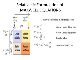
20. Maxwell’s Equations in Relativistic
Formulation
All the four Maxwell equations can be written in
compact form in the following two equations :
𝜕Fμv
𝜕xv
= μ0Jμ
𝜕Gμv
𝜕xv
= 0

21. Gauss’s Law 𝛁. 𝐄 =
𝟏
𝛜 𝟎
𝛒
𝜕F0v
𝜕xv
=
𝜕F00
𝜕x0
+
𝜕F01
𝜕x1
+
𝜕F02
𝜕x2
+
𝜕F03
𝜕x3
=
1
c
𝜕Ex
𝜕x
+
𝜕Ey
𝜕y
+
𝜕Ez
𝜕z
μoJ0
=
1
c
𝛻. E
𝛻. E =
1
ϵ0
ρ which is Gauss’s law.
•

22. Ampere’s Law with Maxwell’s
correction.
𝛻 × 𝐵 = 𝜇 𝑜 𝐽 + 𝜇 𝑜 𝜖0
𝜕𝐸
𝜕𝑡
=>
𝜕𝐹1𝑣
𝜕𝑥 𝑣
=
−1
𝑐2
𝜕𝐸
𝜕𝑡
+ 𝛻 × 𝐵
=> 𝜇 𝑜 𝐽1
= 𝜇 𝑜 𝐽 𝑥 =
−1
𝑐2
𝜕𝐸
𝜕𝑡
+ 𝛻 × 𝐵
Combining this with the corresponding results for 𝜇 =
2 𝑎𝑛𝑑 𝜇 = 3 gives 𝛻 × 𝐵 = 𝜇 𝑜 𝐽 + 𝜇 𝑜 𝜖0
𝜕𝐸
𝜕𝑡
which is
Ampere’s law with Maxwell’s correction.

23. 𝛁. 𝐁 = 𝟎
Using
𝜕Gμv
𝜕xv = 0 and putting μ = 0, and expanding as
above, we get 𝛻. B = 0
Faraday’s Law 𝛁 × 𝐄 = −
𝛛𝐁
𝛛𝐭
Using
𝜕Gμv
𝜕xv = 0 and putting μ = 1, and expanding, we
get
𝛻 × E = −
𝜕B
𝜕t
.

24. References
• Concept of Modern Physics by Arthur Beiser
• Concepts of Physics by H.C Verma
• Introduction to Particle Physics by D.J Griffiths
• Electrodynamics by D.J Griffiths