The document provides mathematical derivations of key concepts in fluid dynamics, including: 1) Definitions of hyperbolic functions like sinh, cosh, and tanh and their basic properties. 2) The fundamental fluid flow equations - continuity, irrotationality/use of a velocity potential, and the time-dependent Bernoulli equation - that are used to model wave behavior. 3) The derivation of the wave field and dispersion relationship by applying Laplace's equation, kinematic and dynamic boundary conditions, and making linear approximations to obtain solutions for a sinusoidal wave.

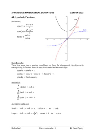
1. Hydraulics 3 Waves: Appendix – 1 Dr David Apsley
APPENDICES: MATHEMATICAL DERIVATIONS AUTUMN 2022
A1. Hyperbolic Functions
Definitions:
sinh(𝑥) ≡
e𝑥
− 𝑒−𝑥
2
cosh(𝑥) ≡
e𝑥
+ 𝑒−𝑥
2
tanh 𝑥 ≡
sinh 𝑥
cosh 𝑥
Basic Formulae
These bear more than a passing resemblance to those for trigonometric functions (with
corresponding definitions for sech, cosech and coth), but beware of signs:
cosh2
𝑥 − sinh2
x = 1
cosh 2𝑥 = cosh2
𝑥 + sinh2
𝑥 = 2 cosh2
𝑥 − 1
sinh 2𝑥 = 2 sinh 𝑥 cosh 𝑥
Derivatives
d
d𝑥
(sinh 𝑥) = cosh 𝑥
d
d𝑥
(cosh 𝑥) = sinh 𝑥
d
d𝑥
(tanh 𝑥) = sech2
𝑥
Asymptotic Behaviour
Small x: sinh 𝑥 ~ tanh 𝑥 ~ 𝑥, cosh 𝑥 → 1 as 𝑥 → 0
Large x: sinh 𝑥 ~ cosh 𝑥 ~
1
2
e𝑥
, tanh 𝑥 → 1 as 𝑥 → ∞

2. Hydraulics 3 Waves: Appendix – 2 Dr David Apsley
A2. Fluid-Flow Equations
To start, we need mathematical equations for three fluid-dynamical principles: continuity,
irrotationality (or, equivalently, use of a velocity potential) and the time-dependent Bernoulli
equation (mechanical energy). In two dimensions, with coordinates (𝑥, 𝑧) and velocity (𝑢, 𝑤),
and assuming incompressible and inviscid flow, these are:
(i) Continuity:
𝜕𝑢
𝜕𝑥
+
𝜕𝑤
𝜕𝑧
= 0
(ii) Irrotationality:
𝜕𝑢
𝜕𝑧
−
𝜕𝑤
𝜕𝑥
= 0 or 𝑢 =
𝜕𝜙
𝜕𝑥
, 𝑤 =
𝜕𝜙
𝜕𝑧
where 𝜙 is a velocity potential.
(iii) Time-dependent Bernoulli equation:
𝜌
∂𝜙
𝜕𝑡
+ 𝑝 +
1
2
𝜌𝑈2
+ 𝜌𝑔𝑧 = 𝐶(𝑡), along a streamline
where 𝑈 is the speed, or magnitude of velocity: 𝑈2
= 𝑢2
+ 𝑤2
.
Heuristic justifications for these follow.
Continuity
Consider flow in the 𝑥 − 𝑧 plane and flow through the sides of a small rectangular control
volume, with sides Δ𝑥, Δ𝑧. In incompressible flow, the net volume flux out of this volume is
zero.
Since the volume flux through any surface is (velocity)  (area) then, per unit depth normal to
this plane, and with the notation in the figure:
net volume outflow = 𝑢𝑒Δ𝑧 − 𝑢𝑤Δ𝑧 + 𝑤𝑛Δ𝑥 − 𝑤𝑠Δ𝑥 = 0
Dividing by area Δ𝑥Δ𝑧:
𝑢𝑒 − 𝑢𝑤
Δ𝑥
+
𝑤𝑛 − 𝑤𝑠
Δ𝑧
= 0
Δ𝑢
Δ𝑥
+
Δ𝑤
Δ𝑧
= 0
In the limit as Δ𝑥, Δ𝑧 → 0:
𝜕𝑢
𝜕𝑥
+
𝜕𝑤
𝜕𝑧
= 0
ue
uw
wn
ws
z
x

3. Hydraulics 3 Waves: Appendix – 3 Dr David Apsley
Irrotationality
Irrotationality is a consequence of the inviscid approximation. In the absence of viscous forces
(and density gradients) the only forces acting on a fluid element are pressure and a constant
gravity force. The former acts perpendicular to the boundary of the element and the latter is
constant, so neither can impart rotation (or “circulation”). Hence (see figure):
circulation(≡ line integral of velocity) = 0
For our 2-d volume, and working clockwise from the top edge:
𝑢𝑛Δ𝑥 − 𝑤𝑒Δ𝑧 − 𝑢𝑠Δ𝑥 + 𝑤𝑤Δ𝑧 = 0
Dividing by area Δ𝑥Δ𝑧:
𝑢𝑛 − 𝑢𝑠
Δ𝑧
−
𝑤𝑒 − 𝑤𝑤
Δ𝑥
= 0
Δ𝑢
Δ𝑧
−
Δ𝑤
Δ𝑥
= 0
In the limit as Δ𝑥, Δ𝑧 → 0:
𝜕𝑢
𝜕𝑧
−
𝜕𝑤
𝜕𝑥
= 0
(1)
If we define the velocity potential 𝜙 as the line integral of velocity from an arbitrary reference
point to (𝑥, 𝑧), then 𝜙 is well-defined because the no-circulation condition makes this
independent of route. In particular, considering the change from bottom-left to top-right of our
representative control volume, by either route, and working directly in infinitesimals:
d𝜙 = 𝑢 d𝑥 + 𝑤 d𝑧
But, comparing the expansion for any 2-d function:
d𝜙 =
𝜕𝜙
𝜕𝑥
d𝑥 +
𝜕𝜙
𝜕𝑧
d𝑧
we have
𝑢 =
𝜕𝜙
𝜕𝑥
, 𝑤 =
𝜕𝜙
𝜕𝑧
As a check, substitute in the LHS of (1) to get
𝜕2
𝜙
𝜕𝑧 𝜕𝑥
−
𝜕2
𝜙
∂𝑥 𝜕𝑧
which vanishes by the symmetry of the second derivatives.
It is convenient to write all flow variables (𝑢, 𝑤, 𝑝) in terms of 𝜙, because we then only have
one equation to solve. However, the ability to do so relies on the assumption of irrotationality
(here, due to the inviscid approximation) which does not hold in, for example, boundary layers.
we
ww
un
us
z
x

4. Hydraulics 3 Waves: Appendix – 4 Dr David Apsley
Time-Dependent Bernoulli Equation
Writing “mass  acceleration = force”, per unit volume, and in the
direction of a streamline:
𝜌 (
𝜕𝑈
𝜕𝑡
+ 𝑈
𝜕𝑈
𝜕𝑠
) = −
𝜕𝑝
𝜕𝑠
− 𝜌𝑔 sin θ
where 𝑈 is the magnitude of velocity, 𝑠 is the distance along a streamline and θ is the angle
between streamline and horizontal.
From trigonometry, sin 𝜃 = Δ𝑧 Δ𝑠
⁄ , or, along a streamline, sin 𝜃 = ∂𝑧 ∂𝑠
⁄ , whilst, in terms of
the velocity potential, 𝑈 = ∂𝜙 ∂𝑠
⁄ . Hence, after rearranging (and assuming ρ constant):
𝜕
𝜕𝑠
[𝜌
𝜕𝜙
𝜕𝑡
+
1
2
𝜌𝑈2
+ 𝑝 + 𝜌𝑔𝑧] = 0
Hence,
𝜌
∂𝜙
𝜕𝑡
+ 𝑝 +
1
2
𝜌𝑈2
+ 𝜌𝑔𝑧 = 𝐶(𝑡), along any particular streamline
We will use the time-dependent version here. However, note that, in the time-steady case, this
reduces to the “normal” Bernoulli equation:
𝑝 + 𝜌𝑔𝑧 +
1
2
𝜌𝑈2
= constant, along a streamline
3-d Generalisations (Not Examinable)
The above are very hand-waving arguments. Far better (but more mathematical) derivations
can be found in any good fluid-mechanics textbook. There are also 3-d generalisations:
Continuity:
∇ •u ≡
𝜕𝑢
𝜕𝑥
+
𝜕𝑣
𝜕𝑦
+
𝜕𝑤
𝜕𝑧
= 0
Irrotationality:
∇˄u ≡
(
𝜕𝑤
𝜕𝑦
−
𝜕𝑣
𝜕𝑧
𝜕𝑢
𝜕𝑧
−
𝜕𝑤
𝜕𝑥
𝜕𝑣
𝜕𝑥
−
𝜕𝑢
𝜕𝑦)
= 0
∇˄u is called vorticity. In this course we are only using the 𝑦 component (i.e. the circulation
in the 𝑥 − 𝑧 plane).
In terms of the velocity potential:

U
s

5. Hydraulics 3 Waves: Appendix – 5 Dr David Apsley
u = ∇𝜙 =
(
𝜕𝜙
𝜕𝑥
𝜕𝜙
𝜕𝑦
𝜕𝜙
𝜕𝑧)
The time-dependent Bernoulli equation is unchanged.

6. Hydraulics 3 Waves: Appendix – 6 Dr David Apsley
A3. Derivation of Wave Field and Dispersion Equation
A3.1 Laplace’s Equation For the Velocity Potential
𝜕2
𝜙
𝜕𝑥2
+
𝜕2
𝜙
𝜕𝑧2
= 0
A3.2 Boundary Conditions
Boundary conditions are applied at the bed and the free surface. These are of two types:
• kinematic (no net flow through a boundary);
• dynamic (stress is continuous at a boundary).
A3.2.1 Kinematic Boundary Conditions
The condition that the curve
𝑧 = 𝑧surf(𝑥, 𝑡)
be a material surface (i.e. that the particles constituting it are always the same; or, there is no
net flow through it) is that the total derivative following the flow (𝑢, 𝑤) satisfies
D
D𝑡
(𝑧 − 𝑧surf) = 0 on 𝑧 = 𝑧surf(𝑥, 𝑡)
where, in 2 dimensions,
D
D𝑡
≡
𝜕
𝜕𝑡
+ 𝑢
𝜕
𝜕𝑥
+ 𝑤
𝜕
𝜕𝑧
Expanding and rearranging:
𝑤 =
𝜕𝑧surf
𝜕𝑡
+ 𝑢
𝜕𝑧surf
𝜕𝑥
on 𝑧 = 𝑧surf(𝑥, 𝑡)
This gives the following kinematic boundary conditions.
Bed (KBBC – Kinematic Bed Boundary Condition)
Assuming the bed is horizontal and rigid:
𝑤 = 0 on 𝑧 = −ℎ
Free Surface (KFSBC – Kinematic Free-Surface Boundary Condition)
𝑤 =
𝜕𝜂
𝜕𝑡
+ 𝑢
𝜕𝜂
𝜕𝑥
on 𝑧 = 𝜂(𝑥, 𝑡)

7. Hydraulics 3 Waves: Appendix – 7 Dr David Apsley
A3.2.2 Dynamic Boundary Conditions
The stress on either side of a surface must be continuous (or the particles constituting the
surface would have infinite acceleration).
Free Surface (DFSBC – Dynamic Free-Surface Boundary Condition)
Neglecting viscosity and surface tension, pressure must be atmospheric at the free surface.
Hence, in terms of gauge pressure:
𝑝 = 0 on 𝑧 = 𝜂(𝑥, 𝑡)
Taken together with Bernoulli’s equation, and noting that the free surface is a streamline,
𝜌
∂𝜙
𝜕𝑡
+
1
2
𝜌𝑈2
+ 𝜌𝑔𝜂 = 𝐶(𝑡) on 𝑧 = 𝜂(𝑥, 𝑡)
No dynamic boundary condition is applied at the bed, which can absorb any pressure
distribution impressed on it.
A3.3 Linearised Equations
When an expression is expanded in terms of a small quantity 𝜀 it is common to drop quadratic
and higher terms. i.e. if
𝑦 = 𝑎 + 𝑏𝜀 + 𝑐𝜀2
+ ⋯
then it is common to neglect terms in 𝜀2
and greater, so leaving the linear terms only:
𝑦 = 𝑎 + 𝑏𝜀
Here, we assume that the wave amplitude 𝐴 is small (compared with depth ℎ and wavelength
𝐿) and hence neglect products and powers above the first of wave-related perturbations.
Moreover, boundary conditions at 𝑧 = 𝜂(𝑥, 𝑡) can effectively be applied at 𝑧 = 0.
With this assumption, the governing equations are the following.
Laplace’s equation for the velocity potential is already linear:
𝜕2
𝜙
𝜕𝑥2
+
𝜕2
𝜙
𝜕𝑧2
= 0
The linearised boundary conditions, written in terms of the velocity potential 𝜙 are:
KBBC:
𝜕𝜙
𝜕𝑧
= 0 on 𝑧 = −ℎ
KFSBC:
𝜕𝜙
𝜕𝑧
=
𝜕𝜂
𝜕𝑡
on 𝑧 = 0

8. Hydraulics 3 Waves: Appendix – 8 Dr David Apsley
DFSBC:
∂𝜙
𝜕𝑡
+ 𝑔𝜂 = 𝐶(𝑡) on 𝑧 = 0
A3.4 Solution for a Sinusoidal Wave
The linearised equations above are to be solved for a surface displacement that is a single
harmonic wave component, noting that, under linearity assumptions, the general solution
would be a sum over individual wave components:
𝜂 = 𝐴 cos(𝑘𝑥 − 𝜔𝑡)
Under appropriate boundary conditions, Laplace’s equation has unique solutions. Look for
separable solutions:
𝜙 = 𝑋(𝑥, 𝑡)𝑍(𝑧)
From the KFSBC:
𝑋
d𝑍
d𝑧
|
𝑧=0
= 𝐴𝜔 sin(𝑘𝑥 − 𝜔𝑡)
Hence, 𝑋 ∝ sin(𝑘𝑥 − ω𝑡) . WLOG, we can take the constant of proportionality as 1 and absorb
the remainder of the multiplier into 𝑍. Hence,
𝑋 = sin(𝑘𝑥 − 𝜔𝑡)
and
d𝑍
d𝑧
|
𝑧=0
= 𝐴𝜔
From Laplace’s equation:
−𝑘2
𝑋𝑍 + 𝑋
d2
𝑍
d𝑧2
= 0
or
d2
𝑍
d𝑧2
= 𝑘2
𝑍
This has general solution:
𝑍 = 𝛼e𝑘𝑧
+ 𝛽e−𝑘𝑧
From the KFSBC above and the KBBC:
d𝑍
d𝑧
= 𝐴𝜔 on 𝑧 = 0
d𝑍
d𝑧
= 0 on 𝑧 = −ℎ

9. Hydraulics 3 Waves: Appendix – 9 Dr David Apsley
These fix α and β to give, after some messy algebra,
𝑍 =
𝐴𝜔
𝑘
cosh 𝑘(ℎ + 𝑧)
sinh 𝑘ℎ
The solution for the whole potential is then
𝜙 =
𝐴𝜔
𝑘
cosh 𝑘(ℎ + 𝑧)
sinh 𝑘ℎ
sin(𝑘𝑥 − 𝜔𝑡)
Finally, we have to satisfy the DFSBC. This will gives a relationship between frequency 𝜔 and
wavenumber 𝑘 (and hence between period 𝑇 and wavelength 𝐿):
−
𝐴𝜔2
𝑘
cosh 𝑘ℎ
sinh 𝑘ℎ
cos(𝑘𝑥 − 𝜔𝑡) + 𝐴𝑔 cos(𝑘𝑥 − 𝜔𝑡) = 𝐶(𝑡)
The LHS has zero spatial mean; hence the RHS must be identically zero. Hence, after dividing
out 𝐴 cos(𝑘𝑥 − 𝜔𝑡) and rearranging, we arrive at the very famous
Dispersion Relationship:
𝜔2
= 𝑔𝑘 tanh 𝑘ℎ
From this last equation,
𝜔
𝑘
= (
𝑔
𝜔
)
sinh 𝑘ℎ
cosh 𝑘ℎ
and so the velocity potential can also be written
Velocity Potential:
𝜙 =
𝐴𝑔
𝜔
cosh 𝑘(ℎ + 𝑧)
cosh 𝑘ℎ
sin(𝑘𝑥 − 𝜔𝑡)
Once the velocity potential and dispersion relation are known, the velocity, pressure and other
quantities follow immediately.
Velocity
𝑢 ≡
𝜕𝜙
𝜕𝑥
=
𝐴𝑔𝑘
𝜔
cosh 𝑘(ℎ + 𝑧)
cosh 𝑘ℎ
cos(𝑘𝑥 − 𝜔𝑡)
𝑤 ≡
𝜕𝜙
𝜕𝑧
=
𝐴𝑔𝑘
𝜔
sinh 𝑘(ℎ + 𝑧)
cosh 𝑘ℎ
sin(𝑘𝑥 − 𝜔𝑡)
Pressure
From the linearised form of Bernoulli’s equation,

10. Hydraulics 3 Waves: Appendix – 10 Dr David Apsley
𝑝 = −𝜌𝑔𝑧 − 𝜌
∂𝜙
𝜕𝑡
= −𝜌𝑔𝑧 + 𝜌𝑔𝐴
cosh 𝑘(ℎ + 𝑧)
cosh 𝑘ℎ
cos(𝑘𝑥 − 𝜔𝑡)
This can also be written
𝑝 = −𝜌𝑔𝑧 + 𝜌𝑔𝜂
cosh 𝑘(ℎ + 𝑧)
cosh 𝑘ℎ
where we have used the specified surface displacement, 𝜂.
Note:
(i) It is common to decompose the pressure field into hydrostatic and hydrodynamic
components:
𝑝 = −𝜌𝑔𝑧
⏟
hydrostatic
+ 𝜌𝑔𝐴
cosh 𝑘(ℎ + 𝑧)
cosh 𝑘ℎ
cos(𝑘𝑥 − 𝜔𝑡)
⏟
hydrodynamic (i.e. wave)
(ii) Both 𝑢 and 𝑝 demonstrate the characteristic depth dependence
cosh 𝑘(ℎ + 𝑧)
cosh 𝑘ℎ
which varies from 1 at the free surface (𝑧 = 0) to
1
cosh 𝑘ℎ
at the bed (𝑧 = −ℎ). If 𝑘ℎ is large (say, 𝑘ℎ > π) then wave disturbances do not reach
the bed.

11. Hydraulics 3 Waves: Appendix – 11 Dr David Apsley
A4. Wave Kinetic and Potential Energy
Kinetic Energy
Wave kinetic energy (per unit horizontal area) is, integrating over the water column:
KE =
1
2
𝜌 ∫ (𝑢2
+ 𝑤2) d𝑧
𝜂
𝑧=−ℎ
The upper limit may be taken as 0 rather than η because of the linear approximation.
From the solution for the velocity components
𝑢2
+ 𝑤2
= (
𝐴𝑔𝑘
𝜔 cosh 𝑘ℎ
)
2
{cosh2
𝑘(ℎ + 𝑧) cos2(𝑘𝑥 − 𝜔𝑡) + sinh2
𝑘(ℎ + 𝑧) sin2(𝑘𝑥 − 𝜔𝑡)}
The average value of both cos2(𝑘𝑥 − 𝜔𝑡) and sin2(𝑘𝑥 − 𝜔𝑡) over a wave cycle is ½. Hence,
the average wave kinetic energy (per unit horizontal area) is
KE =
1
2
𝜌 (
𝐴𝑔𝑘
𝜔 cosh 𝑘ℎ
)
2
×
1
2
∫ {cosh2
𝑘(ℎ + 𝑧) + sinh2
𝑘(ℎ + 𝑧)}d𝑧
0
−ℎ
=
1
2
𝜌 (
𝐴𝑔𝑘
𝜔 cosh 𝑘ℎ
)
2
×
1
2
∫ cosh 2𝑘(ℎ + 𝑧) d𝑧
0
−ℎ
=
1
2
𝜌 (
𝐴𝑔𝑘
𝜔 cosh 𝑘ℎ
)
2
×
1
2
[
sinh 2𝑘(ℎ + 𝑧)
2𝑘
]
−ℎ
0
=
1
2
𝜌 (
𝐴𝑔𝑘
𝜔 cosh 𝑘ℎ
)
2
×
1
2
[
sinh 2𝑘ℎ
2𝑘
]
−ℎ
0
=
1
2
𝜌 (
𝐴𝑔𝑘
𝜔 cosh 𝑘ℎ
)
2
×
1
2
×
2 sinh 𝑘ℎ cosh 𝑘ℎ
2𝑘
=
1
4
𝜌
𝐴2
𝑔2
𝑘
𝜔2
tanh 𝑘ℎ
But, from the dispersion relation, 𝜔2
= 𝑔𝑘 tanh 𝑘ℎ. Hence,
KE =
1
4
𝜌𝑔𝐴2
Potential Energy
The potential energy (per unit horizontal area) is
∫ 𝜌𝑔𝑧 d𝑧
𝜂
𝑧=−ℎ
=
1
2
𝜌𝑔[𝑧2]−ℎ
𝜂
=
1
2
𝜌𝑔(𝜂2
− ℎ2
)
=
1
2
𝜌𝑔𝜂2
+ constant
We are only interested in the wave-varying part of this, and hence the wave potential energy
per unit area is

12. Hydraulics 3 Waves: Appendix – 12 Dr David Apsley
1
2
𝜌𝑔𝐴2
cos2(𝑘𝑥 − 𝜔𝑡)
Again, the average value of cos2(𝑘𝑥 − 𝜔𝑡) is ½. Hence, the average wave potential energy is
PE =
1
4
𝜌𝑔𝐴2

13. Hydraulics 3 Waves: Appendix – 13 Dr David Apsley
A5. Group Velocity
The group velocity (for any wave type) is defined by
𝑐𝑔 ≡
d𝜔
d𝑘
The dispersion relationship for gravity waves on still water is
𝜔2
= 𝑔𝑘 tanh 𝑘ℎ
Differentiating (implicitly) with respect to k:
2𝜔
d𝜔
d𝑘
= 𝑔 tanh 𝑘ℎ + 𝑔𝑘ℎ sech2
𝑘ℎ
=
𝜔2
𝑘
+
𝜔2
tanh 𝑘ℎ
×
ℎ
cosh2 𝑘ℎ
=
𝜔2
𝑘
[1 +
𝑘ℎ
sinh 𝑘ℎ cosh 𝑘ℎ
]
Hence, using sinh 2𝑥 = 2 sinh 𝑥 cosh 𝑥 (note the factor of 2):
d𝜔
d𝑘
=
1
2
[1 +
2𝑘ℎ
sinh 2𝑘ℎ
]
𝜔
𝑘
or
𝑐𝑔 = 𝑛𝑐
where
𝑐 ≡
𝜔
𝑘
is the phase velocity and
𝑛 =
1
2
[1 +
2𝑘ℎ
sinh 2𝑘ℎ
]
is the ratio of group to phase velocities.

14. Hydraulics 3 Waves: Appendix – 14 Dr David Apsley
A6. Wave Power
The wave power is the (time-averaged) rate of working of pressure forces over a vertical
surface. Integrating over the water column, per unit length of wave crest,
power = ∫ 𝑝𝑢 d𝑧
𝜂
𝑧=−ℎ
We need only consider the hydrodynamic part of 𝑝, since the time-steady hydrostatic part will,
in conjunction with 𝑢, give a component integrating to 0 over a cycle. Using the linear wave
theory expressions for 𝑝 (hydrodynamic) and 𝑢,
𝑝𝑢 = 𝜌𝑔𝐴
cosh 𝑘(ℎ + 𝑧)
cosh 𝑘ℎ
cos(𝑘𝑥 − 𝜔𝑡) ×
𝐴𝑔𝑘
𝜔
cosh 𝑘(ℎ + 𝑧)
cosh 𝑘ℎ
cos(𝑘𝑥 − 𝜔𝑡)
=
𝜌𝑔2
𝐴2
𝑘
𝜔
cosh2
𝑘(ℎ + 𝑧)
cosh2 𝑘ℎ
cos2
(𝑘𝑥 − 𝜔𝑡)
Under the linear approximation, the upper limit of integration may be replaced by 𝑧 = 0.
The average value of cos2(𝑘𝑥 − 𝜔𝑡) is ½, whilst integrating the 𝑧-dependent part over the
water column gives
∫ cosh2
𝑘(ℎ + 𝑧) d𝑧
0
−ℎ
=
1
2
∫ (cosh 2𝑘(ℎ + 𝑧) + 1) d𝑧
0
−ℎ
=
1
2
[
sinh 2𝑘(ℎ + 𝑧)
2𝑘
+ 𝑧]
−ℎ
0
=
1
2
(
sinh 2𝑘ℎ
2𝑘
+ ℎ)
Hence, the wave power is
𝑃 =
𝜌𝑔2
𝑘𝐴2
𝜔 cosh2 𝑘ℎ
×
1
2
(
sinh 2𝑘ℎ
2𝑘
+ ℎ) ×
1
2
=
1
2
𝜌𝑔𝐴2
×
𝑔𝑘
𝜔 cosh2 𝑘ℎ
×
sinh 2𝑘ℎ
2𝑘
(1 +
2𝑘ℎ
sinh 2𝑘ℎ
) ×
1
2
=
1
2
𝜌𝑔𝐴2
×
𝑔𝑘
𝜔 cosh2 𝑘ℎ
×
2 sinh 𝑘ℎ cosh 𝑘ℎ
2𝑘
× (1 +
2𝑘ℎ
sinh 2𝑘ℎ
) ×
1
2
=
1
2
𝜌𝑔𝐴2
× (
𝑔𝑘 tanh 𝑘ℎ
𝜔2
) ×
1
2
(1 +
2𝑘ℎ
sinh 2𝑘ℎ
)
𝜔
𝑘
But the wave energy density is
𝐸 =
1
2
𝜌𝑔𝐴2
the dispersion relationship is
𝜔2
= 𝑔𝑘 tanh 𝑘ℎ
and the group velocity
𝑐𝑔 = 𝑛𝑐

15. Hydraulics 3 Waves: Appendix – 15 Dr David Apsley
where
𝑛 =
1
2
(1 +
2𝑘ℎ
sinh 2𝑘ℎ
) , 𝑐 =
𝜔
𝑘
Hence, the wave power per unit length of crest is
𝑃 = 𝐸𝑐𝑔