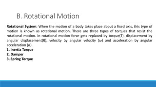
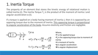
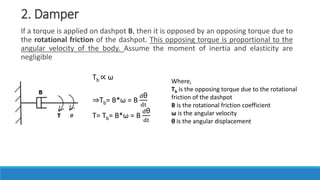
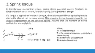
Downloaded 19 times


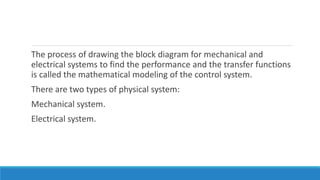
![2. Spring Force:
We all have seen spring and we know how it contracts and retracts on application of force.
A mechanical system could have an actual spring or spring like component in it e.g. belt or cable.
Springs are non linear device but their deformation is linear for short distance.
Consider a spring shown in figure
We require force to deform the spring . Here the force is proportional to the displacement.
Net displacement of application of force F(t) at end A is x1 - x2
Therefore, F(t) = K[x1 (t) –x2 (t)]
If the force is applied at B end the relationship is
1
x2
A
B
F(t) = K[x2 (t) –x1 (t)]
Applying Laplace Transform
F(s) = K[X1 (s) –X2 (s)]
• K '= spring constant of stiffness](https://image.slidesharecdn.com/unit1acs-231219061805-f6a6888c/85/Introduction-to-Automatic-Control-Systems-48-320.jpg)
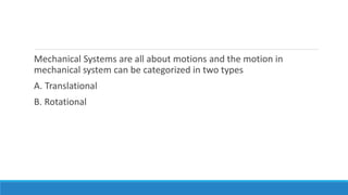
![3. Damping Force/ Friction:
Whenever there is motion there exist friction. Friction exists between moving body and a
fixed support or between surfaces. Sometime viscous friction is sometimes introduced
intentionally which is shown as dashpot or damper.
For viscous friction, we assume that the damping force is proportional to the velocity.
2
x1
FD(t) = B
𝒅
𝒅𝒕
[x1(t) –x2(t)]
Applying Laplace FD(s) = Bs [X2 (s) –X1 (s)]](https://image.slidesharecdn.com/unit1acs-231219061805-f6a6888c/85/Introduction-to-Automatic-Control-Systems-49-320.jpg)
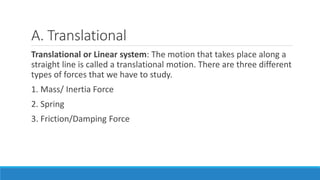
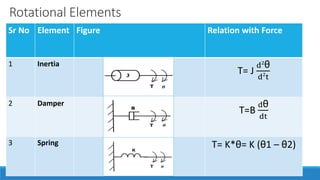
![Translational Elements
Sr No Element Figure Relation with Force
1 Mass
2 Spring
3 Friction
M F (t)
x
1
x2
A
B
2
x1
F(t) = K[x1 (t) –x2 (t)]
FD(t) = B
𝒅
𝒅𝒕
[x1 (t) –x2 (t)]](https://image.slidesharecdn.com/unit1acs-231219061805-f6a6888c/85/Introduction-to-Automatic-Control-Systems-54-320.jpg)
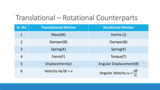
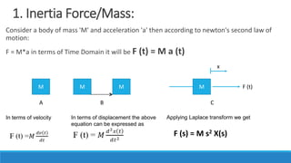
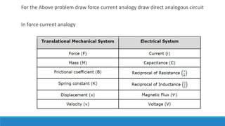
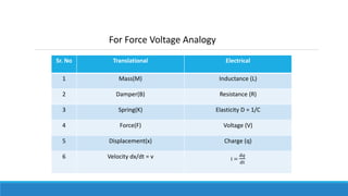
![Translational
Mechanical System
Equation Figure Electrical System Equation Figure
Input- Force (F) F = m a Input- Voltage (V) V = I R
Output- Velocity (v) Output- Current (i)
Mass (M) Inductance (L) v=L
di
dt
Damper/Friction
(B)
FD= B
𝒅
𝒅𝒕
[x1–x2] Resistance(R) v= i R
Spring (K) F = K[x1 –x2 ] Reciprocal of
Capacitance (1/𝐶)
v =
1
C
∫ idt
Displacement (x) Charge (q)
M F (t) i(t)
v(t)
2 x1
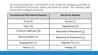
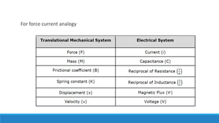
By comparing Equation 1 and Equation 3, we will get the analogous quantities of the translational
mechanical system and electrical system. The following table shows these analogous quantities.](https://image.slidesharecdn.com/unit1acs-231219061805-f6a6888c/85/Introduction-to-Automatic-Control-Systems-61-320.jpg)
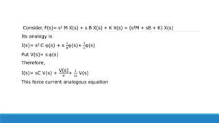

![Its analogy is
I(s)= s2 C1ϕ1(s) +
1
𝐿1
ϕ1 (s) + s
1
𝑅1
ϕ1 (s) +
1
𝐿2
[ϕ1 (s) – ϕ2 (s)]
Put V(s)= s ϕ(s)
Therefore,
I(s)= sC1 V1(s) +
1
𝑠𝐿1
V1(s) +
V1(s)
𝑅1
+
1
𝑠𝐿2
[V1 (s) – V2 (s)]-------------3
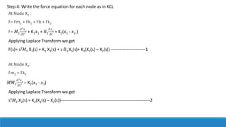
This force current analogous equation for equation number 1
Consider, Equation no 1
F(s)= s2 𝑀1 X1(s) + K1 X1(s) + s 𝐵1 X1(s)+ K2(X1(s) – X2(s))](https://image.slidesharecdn.com/unit1acs-231219061805-f6a6888c/85/Introduction-to-Automatic-Control-Systems-79-320.jpg)
![Its analogy is
s2 C2ϕ2(s) =
1
𝐿2
[ϕ1 (s) – ϕ2 (s)]
Put V(s)= s ϕ(s)
Therefore,
sC2 V2(s) =
1
𝑠𝐿2
[V1 (s) – V2 (s)]----------------------4
This force current analogous equation for equation number 2
Consider, Equation no 2
s2 𝑀2 X2(s) = K2(X1(s) – X2(s))](https://image.slidesharecdn.com/unit1acs-231219061805-f6a6888c/85/Introduction-to-Automatic-Control-Systems-80-320.jpg)
![Its analogy is
V(s)= s2 L1q1(s) +
1
𝐶1
q1 (s) + s 𝑅1 q1 (s) +
1
𝐶2
[q1 (s) – q2 (s)]
Put I(s)= sq(s)
Therefore,
V(s)= sL1 I1(s) +
1
𝑠𝐶1
I1(s) + R1I1 (s) +
1
𝑠𝐶2
[I1 (s) – I2 (s)]----------------5
This force voltage analogous equation for equation number 1
Consider, Equation no 1
F(s)= s2 𝑀1 X1(s) + K1 X1(s) + s 𝐵1 X1(s)+ K2(X1(s) – X2(s))](https://image.slidesharecdn.com/unit1acs-231219061805-f6a6888c/85/Introduction-to-Automatic-Control-Systems-83-320.jpg)
![Its analogy is
s2 L2q2(s) =
1
𝐶2
[q1 (s) – q2 (s)]
Put I(s)= sq(s)
Therefore,
sL2I2(s) =
1
𝑠𝐶2
[I1 (s) – I2 (s)]---------------------6
This force voltage analogous equation for equation number 2
Consider, Equation no 2
s2 𝑀2 X2(s) = K2(X1(s) – X2(s))](https://image.slidesharecdn.com/unit1acs-231219061805-f6a6888c/85/Introduction-to-Automatic-Control-Systems-84-320.jpg)
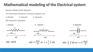
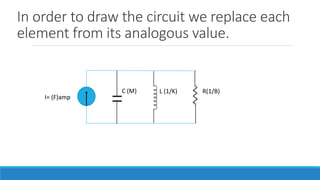
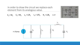
![In order to draw the circuit we replace each
element from its analogous value.
V= (F)volt
C1
L1 R1
C1 = 1/K1 C2 = 1/K2
L1 =M1 L2 = M2 R1 = B1 V = F
C2
L2
I1
Consider eq 5
V(s)= sL1 I1(s) +
1
𝑠𝐶1
I1(s) + R1I1 (s) +
1
𝑠𝐶2
[I1 (s) – I2 (s)]
I1 Flow in C1, R1, L1 hence they are in series.
I1 and I2 flows in C2 hence C2 is common both.
I2 flows in L2 . Hence from above conclusions we draw the circuit](https://image.slidesharecdn.com/unit1acs-231219061805-f6a6888c/85/Introduction-to-Automatic-Control-Systems-85-320.jpg)

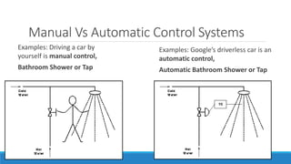
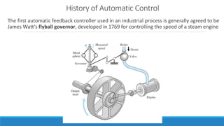
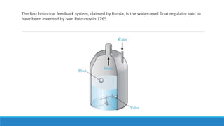
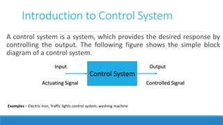
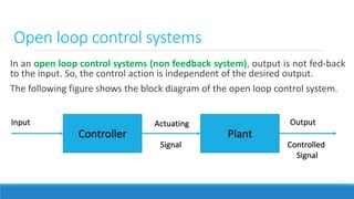
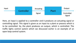
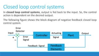
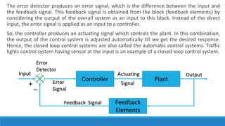
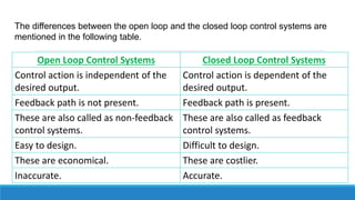
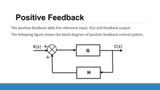
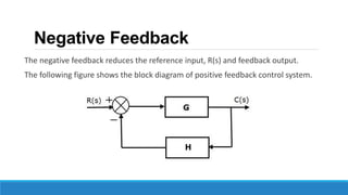
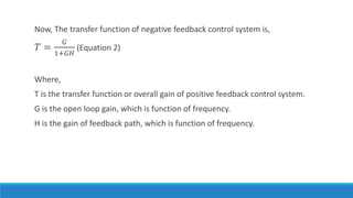
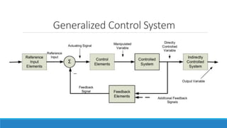
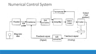
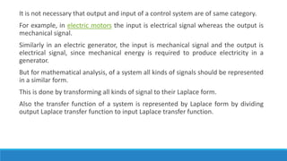
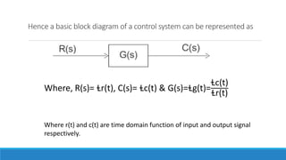
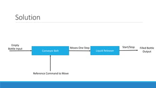
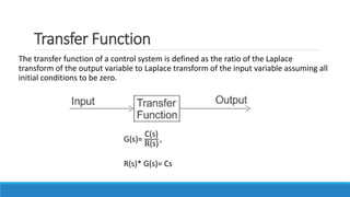
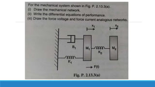
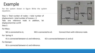
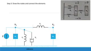
The document provides an introduction to automatic control systems. It discusses: 1. The objectives of understanding basic control concepts, mathematical modeling using block diagrams, and studying systems in time and frequency domains. 2. The differences between manual and automatic control systems, with examples of driverless cars versus manual driving. 3. A brief history of automatic control, including James Watt's flyball governor and Ivan Polzunov's water-level regulator. 4. An overview of control system components and their representation in block diagrams.


![PLC Ladder Programming [Mechatronics]](https://cdn.slidesharecdn.com/ss_thumbnails/plc-ppt-snteli-200503070616-thumbnail.jpg?width=640&height=640&fit=bounds)