The document discusses environmental stress screening (ESS) processes used to test electronic products and remove latent defects. It notes that while ESS is commonly used, failure rate analysis is not always performed to evaluate screening effectiveness. The document recommends analyzing failure rate distributions over time using the Chance Defective Exponential model to determine optimal ESS screening times and ensure high outgoing quality. Adaptive ESS processes that adjust screening parameters based on results can further reduce defects.

1. Hilaire Ananda Perera
Long Term Quality Assurance
http://www.linkedin.com/in/hilaireperera
Outgoing Reliability Assurance of “End-
Units” using the Chance Defective
Exponential (CDE) Model
“Taguchi said that the Loss to Society increases as the value of a
quality characteristic (i.e. Defect Density, Failure Rate, etc.) departs
from the optimal value.”
Environmental Stress Screening (ESS) is performed on most of the
Electronic/Electrical products. However failure rate/time distribution
analysis is not conducted always to evaluate the effectiveness of
the Screening Process. We have placed too much emphasis on the
Mean Time Between Failure (MTBF), and have ignored this
valuable process to monitor and assure the Outgoing Reliability of
our products
Page 1

2. Hilaire Ananda Perera
Long Term Quality Assurance
http://www.linkedin.com/in/hilaireperera
The Adaptive Environmental Stress (ESS)
Screening Process
SUMMARY TO OTHER SCREENING
PROGRAMS
SUMMARY TO OTHER PROGRAM
MANAGERS
IDENTIFY
SCREENING
GOALS
DEVELOP
SCREENING
PLANS
INDUSTRY
EXPERIENCE
OTHER
PROGRAM
EXPERIENCE
ASSESS
IMPACT
FAVOURABLE
IMPACT?
SUMMARY TO PROGRAM
MANAGER
SUMMARY TO QUALITY /
RELIABILITY MANAGERS
CONTINUE
OR REDUCE
SCREENING
SCREENING
GOAL MET?
EFFECTIVENESS
REVIEW
DEVELOP
FACILITIES
SPECIFICATIONS
ACQUIRE OR
MODIFY TEST
FACILITIES
SPECIAL TESTS
FOR FACILITIES
OR TOOLS
DEVELOP
DETAILED
PROCEDURES
INCORPORATE
IN ATPs
DEFINE DATA
REQUIREMENTS
ORGANIZE DATA
COLLECTION
RESOURCES
COLLECT DATA
FOR
EFFECTIVENESS
REVIEW
IMPLEMENT
SCREEN
PHASE 1
PHASE 2
PHASE 3
Yes
No
Yes
No
ESS is a process rather than a test in the normal accept/reject sense. Adaptive ESS is
based on the adjustment of screens in response to previously observed screening
results to minimize outgoing defects. With no firm failure mechanism/mode information,
Random Vibration followed by Thermal Cycling with few Power On/Off cycles is a good
default stress condition. Screening should not stress the equipment such that fatigue
failures are precipitated. Contract terms should be flexible enough to permit
modifications of screen parameters when such modifications can be shown to be
beneficial.
Page 2

3. Hilaire Ananda Perera
Long Term Quality Assurance
http://www.linkedin.com/in/hilaireperera
Accelerated Life
Environmental Stress Screening
ESS
Failure
Rate (FR)
FR(t) = A + Be
-Ct
X
X
X
X
X
OUTGOING RELIABILITY ASSURANCE
C = Average rate of defect precipitation under a given set of stress conditions
B/C = Incoming Defect Density (Din)
Time
t1 (variable)
Gather failure data and establish failure rate/time distribution functions
Starting t1 is based on equipment parts count. t1 is varied depending on the
effectiveness of the Stress Screen ( Adaptive ESS )
With proper screening levels assure that there are no manufacturing process
related failures. and latent defects ( i.e. ESS + FFT )
Performance of FFT is an accurate precursor to the kind of reliability
to be expected in the field
FFT = Failure Free Time
A / Normal Failure Rate = Acceleration Factor (AF)
Screening Strength (SS) = 1 - e
-Ct
Test Strength (TS) = SS * Detection Efficiency (DE)
Outgoing Defect Density (Dout) = Din * (1 - TS)
Time To Remove 99.999% Defects = (-1/C)*ln (0.00001)
Chance Defective Exponential Model
Page 3

4. Hilaire Ananda Perera
Long Term Quality Assurance
http://www.linkedin.com/in/hilaireperera
Chance Defective Exponential (CDE)
Model
CDE Model is based on the assumption that the population of
components within a lot of like equipments is comprised of two
subpopulations i.e. A main subpopulation of “good” components
and a much smaller subpopulation of defectives.
The defectives contain major flaws which degrade with stress
and time and are manifested as early-life (infant mortality)
failures. The failure rate of a defective component is several
orders of magnitude greater than the failure rate of a “good”
component. Therefore a relatively few defective components can
dominate the reliability of the equipment during early product
life
Page 4

5. Hilaire Ananda Perera
Long Term Quality Assurance
http://www.linkedin.com/in/hilaireperera
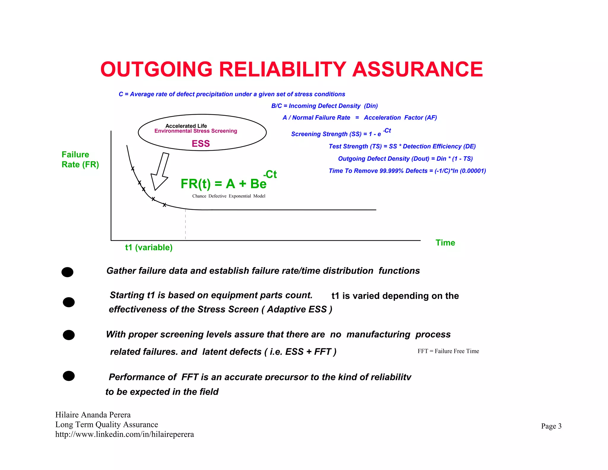
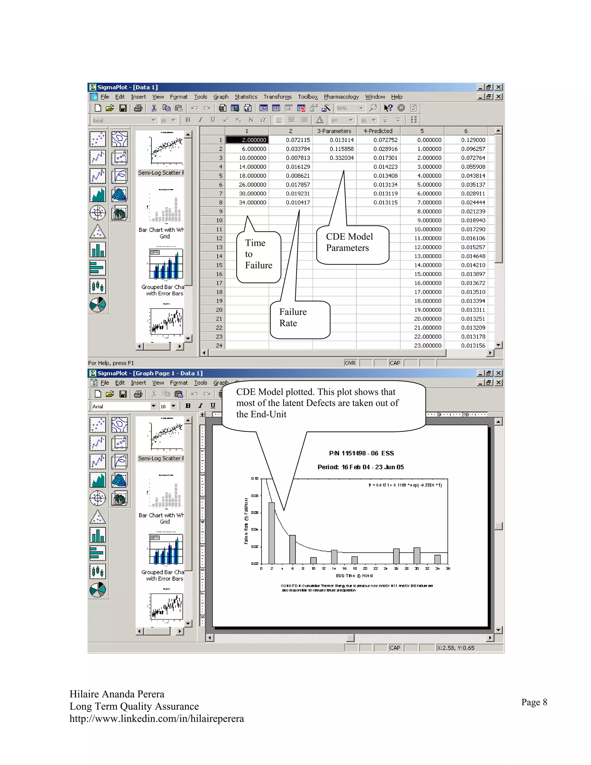
EXAMPLE: Based on the Average Rate of Defect Precipitation of 0.3320 (For
details see Page 8) Defects/Hour, the Time To Remove 99.999% Defects is 34
Hours
NOTE 1: For multiple Screen Stops in a single unit, assume Total Cumulative Thermal
Energy during “No Fault Found (NFF)” and/or “Burn-in Equipment (BIE)” failure
and for true failure responsible for failure precipitation.
Task Sequence for ESS (Thermal Cycling) Failure Rate Distribution
Analysis to Determine the Best Thermal Cycling Time
ESS Failure Data in
Thermal Cycling
Establish Time To Failure
Data Points (Note 1)
Establish Failure/Time
Distribution
Establish Failure
Rate/Time Distribution
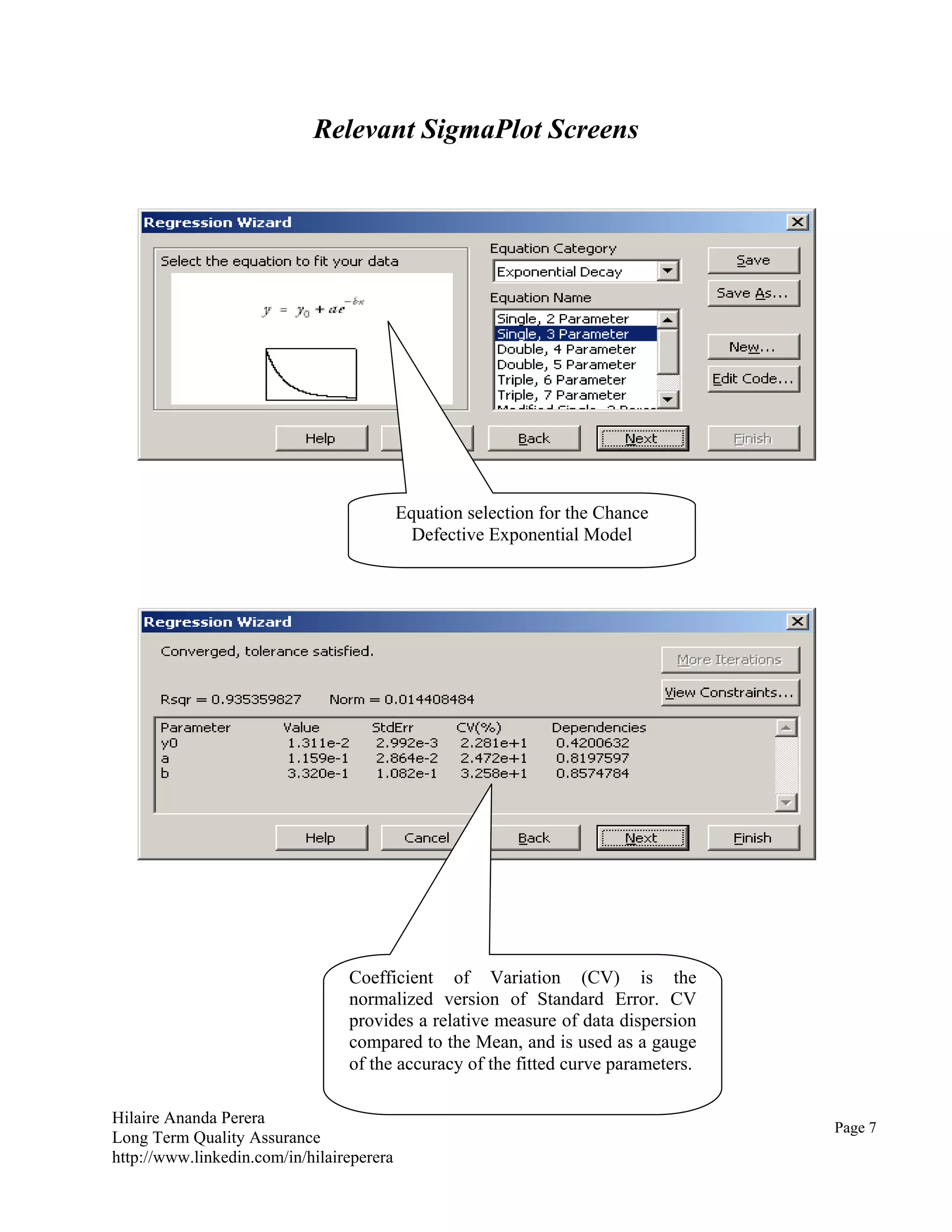
Curve FIT The CDE [A + B*exp(-C*t)] Model
Reference MIL-HDBK-344A
Using SigmaPlot Software Package
Examine the Goodness of Curve Fit Using
Coefficient of Variation (CV) of parameters A,B,C
Determine Time To Remove 99.999% Defects
See
Appendix A
Page 5

6. Hilaire Ananda Perera
Long Term Quality Assurance
http://www.linkedin.com/in/hilaireperera
What SigmaPlot can Do
Page 6

7. Hilaire Ananda Perera
Long Term Quality Assurance
http://www.linkedin.com/in/hilaireperera
Relevant SigmaPlot Screens
Relevant SigmaPlot Screens
Coefficient of Variation (CV) is the
normalized version of Standard Error. CV
provides a relative measure of data dispersion
compared to the Mean, and is used as a gauge
of the accuracy of the fitted curve parameters.
Equation selection for the Chance
Defective Exponential Model
Page 7

8. Hilaire Ananda Perera
Long Term Quality Assurance
http://www.linkedin.com/in/hilaireperera
Time
to
Failure
Failure
Rate
CDE Model
Parameters
CDE Model plotted. This plot shows that
most of the latent Defects are taken out of
the End-Unit
Page 8

9. Hilaire Ananda Perera
Long Term Quality Assurance
http://www.linkedin.com/in/hilaireperera
Control The Consumption of Useful Life
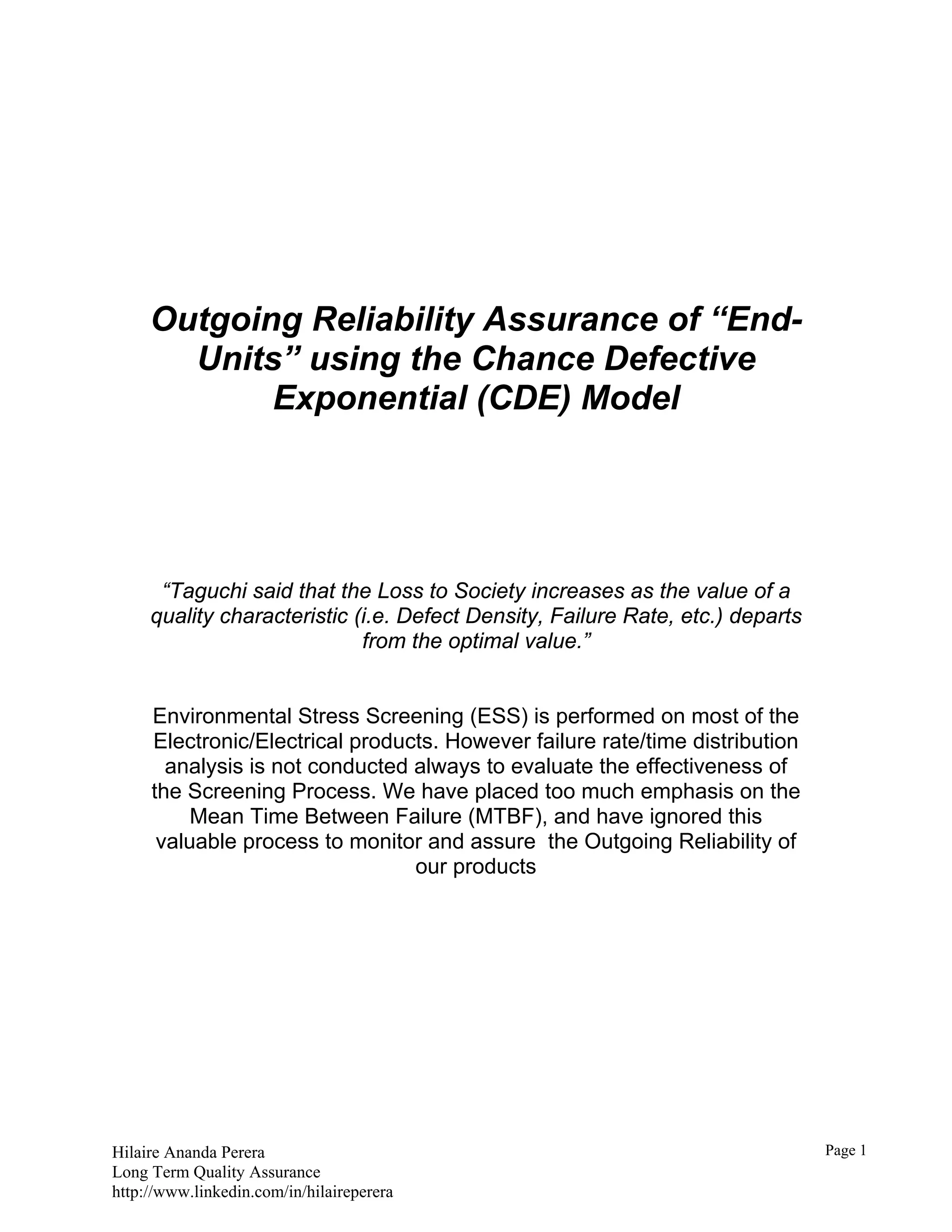
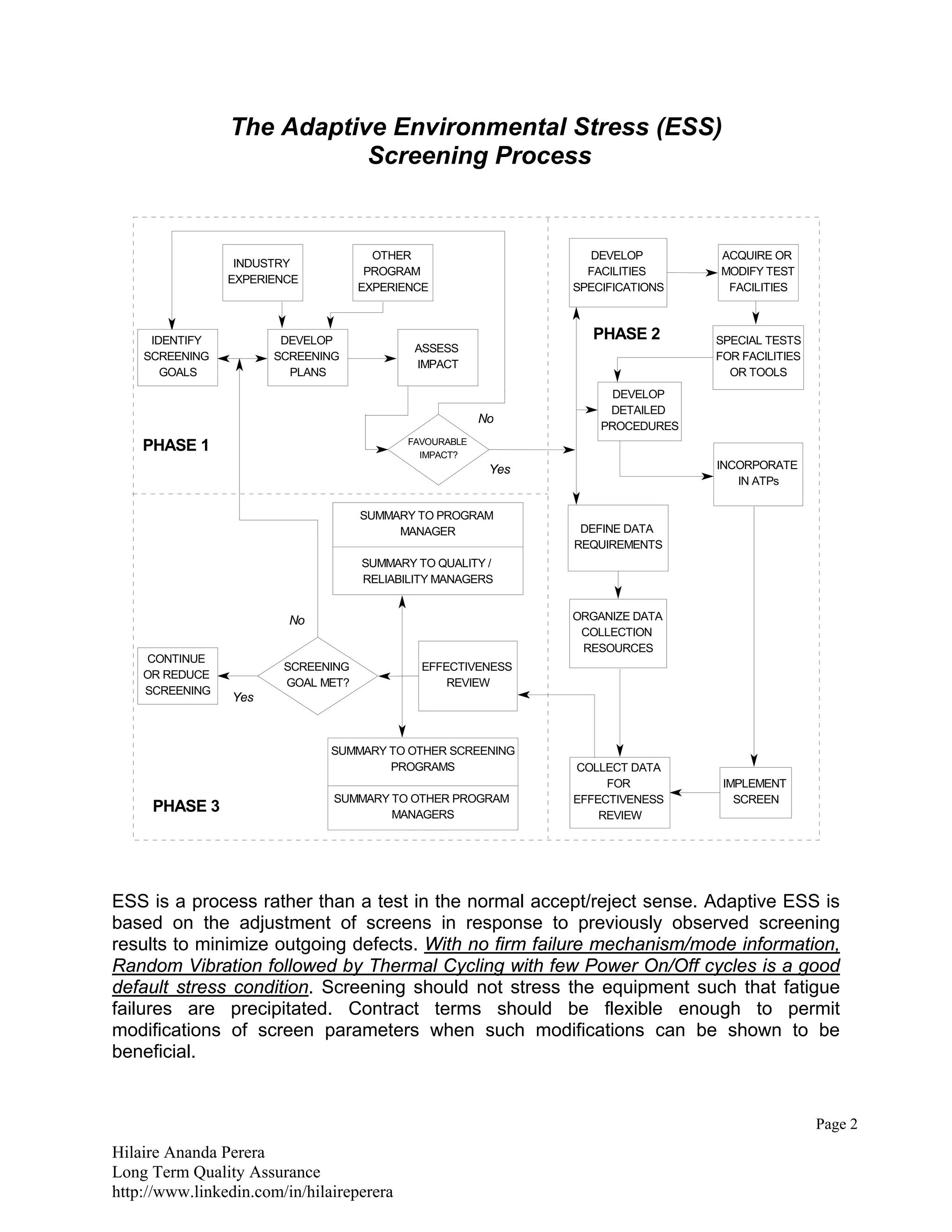
The purpose of the Environmental Stress Screening (ESS) process is to remove latent defects
without consuming an unacceptable portion of the “End-Unit” Useful Life. A common practice
in thermal cycling ESS is to require the last cycle, or the last two or three (usually the number of
cycles are based on the % of failed components) to be failure free with no limit placed on the
maximum number of cycles to which the product is subjected. If a failure occurs in a cycle that is
required to be failure free, the appropriate corrective action is performed and the cycle is
repeated. Thus the failure of one element, such as a component or connection, of a system causes
the entire system to be subjected to additional cycles. The following shows how to control the
consumption of useful life
Acceleration Factor (AF) =
RateFailurePredicted
CurveESSofRateFailureConstant
NOTE: When a high confidence field failure rate is obtained, do not use the predicted failure rate to get the true AF
estimate
Allowable Cumulative ESS Time for Multiple Repairs
=
AF
ESSforAllowableLifeUsefulMax.%*Hr)(OpLifeUseful
Page 9

10. Hilaire Ananda Perera
Long Term Quality Assurance
http://www.linkedin.com/in/hilaireperera
APPENDIX A
A METHOD FOR FAILURE RATE CALCULATION
A.1 AVERAGE FAILURE RATE ESTIMATE
For any age t, the average failure rate estimate  itˆ at that age, for a
homogeneous sample of identical units which are being subjected to a reliability
test while functioning in the same application and operation environment, is given
by the formula:
 itˆ =
 
 
N t
N t t
f
T i


where;
Nf (t) = Number of units failing in the age increment t or on the time period
from age ti to ti + t.
NT (ti) = Number of units in test, or under observation at the beginning (by
definition) of the age increment t or at age ti.
t = Age increment after ti, during which Nf (t) units fail.
A.2 DATA GATHERING FORMAT
(a) Divide the time axis into suitable time increments, 2 hour increments (If
Thermal Cycle is 2 Hours) are suggested, starting from time 0
(b) Plot a scatter diagram of failures as they occur during the test
(c) Count the number of failures in each time slot and calculate the failure rate
according to the equation in paragraph A.1
(d) Tabulate the failure rate  itˆ and elapsed failure times (ti) taking the mid
point of each time slot as the point estimate of the failure time
Page 10