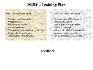
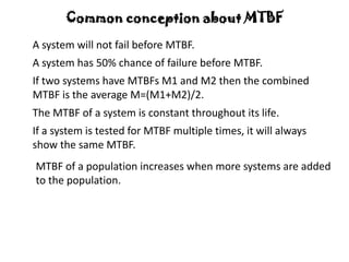
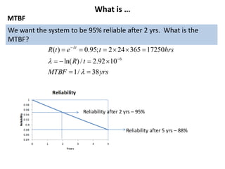
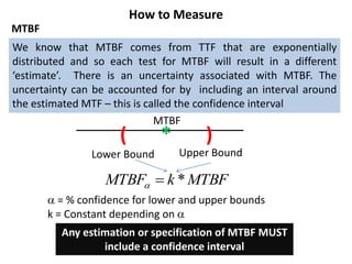
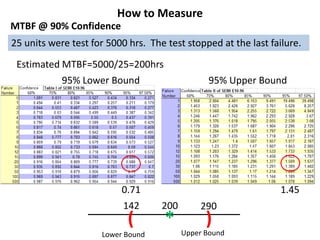
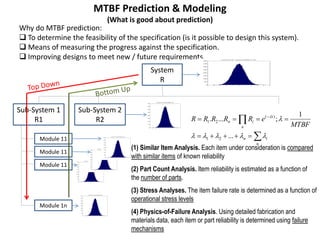
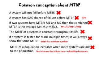
The document discusses MTBF (mean time between failures), including how to calculate, predict, and test it. It addresses common misconceptions about MTBF and describes a two-day training plan that covers the basics of MTBF as well as how to analyze MTBF reports and predictions. The training provides answers to questions and considers reliability modeling techniques to estimate component and system-level MTBF.

1. The MTFB …
What, Why, How and What for.
(and other ins and outs)
Ghulam Mustafa, Ph. D.
©2016

2. MTBF – Training Plan
Day 1: All About the MTBF
- Common mis/conceptions.
- What is MTBF?
- How is it calculated?
- How is it predicted?
- What can be done with the prediction?
- Answers to the questions.
- Some further considerations.
Day 2: On the MTBF Report
- Assumptions of the Report.
- Data and Analysis.
- What actions can be taken?
- What is missing?
- How to do a MTBF prediction?
- Answers to the questions.
- Some further considerations.
Feedback

3. Common conception about MTBF
A system will not fail before MTBF.
A system has 50% chance of failure before MTBF.
If two systems have MTBFs M1 and M2 then the combined
MTBF is the average M=(M1+M2)/2.
The MTBF of a system is constant throughout its life.
If a system is tested for MTBF multiple times, it will always
show the same MTBF.
MTBF of a population increases when more systems are added
to the population.

4. Life’s Big Question
1) Have a good definition of what x is – narrow it down to basics.
2) Find a way to quantify the uncertainty as it relates to x.
Yogi Berra
It’s tough to make predictions,
about the future.
Life … is uncertain. Then x happens. (x=failure event)
MTBF
As far as the laws of mathematics refer to reality, they are not
certain; and as far as they are certain, they do not refer to reality.
Albert Einstein
accurate

5. MTBF – Test Scenario
During a reliability test, 25 units were tested. Time to failure for each unit was recorded. The test was
stopped at the last failure. The test was repeated 3 times.
Inst. MTBF v Failures
Confidence in MTBF estimate
Improves with more testing
Prob(t<MTBF)

6. MTBF – Scenario – Observations / Conclusions
0 200 400 600 800 1000
0
0.1
0.2
0.3
0.4
0.5
0.6
0.7
0.8
0.9
1
Time
0 200 400 600 800 1000
0
0.1
0.2
0.3
0.4
0.5
0.6
0.7
0.8
0.9
1
Time
Artifact of Random Sampling
1. Each test results in a different value of MTBF.
2. Number of times the system fails before MTBF is greater than 50%.
3. Instantaneous MTBF stabilizes with failures (or longer test times)
Observations
1. MTBF is a random variable (with certain characteristics).
2. The probability that the system will fail before MTBF is 63%.
3. Confidence in MTBF increases with failures or longer test time.
Conclusions
Each failure is a sample drawn
from a distribution

7. What is …
MTBF
It is the mean (or the expected value) of the random variable – time
to failure (TTF). TTF is assumed to be exponentially distributed. This
means that the histogram of TTF is an exponential function.
0 0.01 0.02 0.03 0.04 0.05 0.06
0
200
400
600
800
1000
1200
1400
1600
TimetoFailure

1


n
t
MTBF i
=Failure Rate
(failures/hour)
Reliability
It is the probability that system will perform its intended function
for the specified period of time under stated conditions.
368.0)( )(
  MTBFt
eetR 
63.2% chance the system will fail before MTBF

8. What is …
MTBF – 37% Reliable
Reliability after
5 yrs – 5%
Reliability after 1 yr – 62%
Reliability after 6 mo– 78%
MTBF
The MTBF of a unit was determined to be 2 year – how reliable is it?

9. What is …
MTBF
We want the system to be 95% reliable after 2 yrs. What is the
MTBF?
yrsMTBF
tR
hrstetR t
38/1
1092.2/)ln(
17250365242;95.0)(
6








Reliability after 2 yrs – 95%
Reliability after 5 yrs – 88%

10. How to Measure
MTBF
We know that MTBF comes from TTF that are exponentially
distributed and so each test for MTBF will result in a different
‘estimate’. There is an uncertainty associated with MTBF. The
uncertainty can be accounted for by including an interval around
the estimated MTF – this is called the confidence interval
Any estimation or specification of MTBF MUST
include a confidence interval
MTBFkMTBF *
( * )
MTBF
Lower Bound Upper Bound
 = % confidence for lower and upper bounds
k = Constant depending on 

11. How to Measure
MTBF @ 90% Confidence
25 units were test for 5000 hrs. The test stopped at the last failure.
Estimated MTBF=5000/25=200hrs
95% Lower Bound 95% Upper Bound
1.450.71
200
( * )
Lower Bound Upper Bound
142 290

12. MTBF Prediction & Modeling
(What is good about prediction)
Why do MTBF prediction:
 To determine the feasibility of the specification (is it possible to design this system).
 Means of measuring the progress against the specification.
 Improving designs to meet new / future requirements.
System
R
Sub-System 1
R1
Sub-System 2
R2
Module 11
Module 11
Module 11
Module 1n



 
n
in
t
n
in
MTBF
eRRRRR


...
1
;....
21
)(
21
(1) Similar Item Analysis. Each item under consideration is compared
with similar items of known reliability
(2) Part Count Analysis. Item reliability is estimated as a function of
the number of parts.
(3) Stress Analyses. The item failure rate is determined as a function of
operational stress levels
(4) Physics-of-Failure Analysis. Using detailed fabrication and
materials data, each item or part reliability is determined using failure
mechanisms

13. MTBF Prediction & Modeling
(What is good about prediction)
Why do MTBF prediction:
 To determine the feasibility of the specification (is it possible to design this system).
 Means of measuring the progress against the specification.
 Improving designs to meet new / future requirements.
System
R
Sub-System 1
R1
Sub-System 2
R2
Module 11
Module 11
Module 11
Module 1n
Distribution Application
Normal 1- Failure due to wear, such as mechanical devices.
2- Manufacturing varaibility
Log Normal 1- Reliability analysis of semiconductors
2- Fatigue life of certain types of mechanical components
3- Maintainability analysis
Exponential 1- Reliability prediction of electronic equipment
2- Items whose failure rate does not change significantly with
age
3- Complex repairable equipment without excessive
redundancy
4- Equipment for which the "infant mortalities" have been
eliminated by "burning in"
Gamma 1- Cases where partial failures exist (e.g., redundant systems)
2- Time to second failure when the time to failure is
exponentially distributed.
Weibull General distribution which can model a wide range of life
distributions of different classes of engineered items.

14. MTBF Prediction & Modeling
(What is good about prediction)
System
R
Sub-System 1
R1
Sub-System 2
R2
Sub-System n
R5
Module 11
Module 12
Module 13
Module 10



 
n
in
t
n
in
MTBF
eRRRRR


...
1
;....
21
)(
21
=0.001
=0.001
=0.001
=0.001
=0.01
MTBF1000
MTBF1000
MTBF1000
MTBF1000
MTBF100
MTBF20

15. customer cassettes
Operator interface
Wafer aligner
Dual arm robot
Robot track
Processor Electronics rack WhisperScan Beamstop Vacuum chamber
Maintenance
interface
Vacuum robot Single wafer
loadlocks
PFS flange
Injector Booster Beamline Processor Factory Interface
We need system and module boundaries
Reliability Block Diagram

16. 16 |
Reliability Block Diagram
System
(100%)
Carousel
(10%)
Shuttle
(35%)
Gripper
(17%)
Shuttle Horizontal
Drive
(10%)
Active Ports
(15%)
Controls
(10%)
DARTS Sys
Cont.
FAB Int.
Cont.
Drive
Track
FOUP Sensing
Belt Lift
Belt Take-up
Com/PWR Wiring
Shuttle Cont PCB
Interlocks
Controller
Grip Mech.
Sensors.
Interlocks
Drive
Rail Guides
Flex Cable
Control PCB
Vert. Drive
Horizontal Dr.
E84 Func.
Motion Cont.
By-Pass Mode
I/O Board
Ethernet Switch
SW
Stationary Shelf
(3%)
FOUP Sensing
RF ID
Connector Board
(%) is the module failure contribution to the system

17. MTBF in Closed-Loop Feedback
(What is good about prediction)
MTBF prediction sets the goal for product
reliability.
Step 1: Predict MTBF of the system under design.
Step 2: Design the system to meet the MTBF.
Step 3: Test the system to verify design and MTBF.
Step 4: Is the MTBF goal met?
Step 5: Perform F/A and take corrective actions.
Step 6: Repeat 3-5 until D=0.
System
Under Test
(Field Operation)
D Measured
MTBF
Failure Analysis
Corrective Actions
Predicted
MTBF

18. Failure in Electronic Components

19. Failure in Incandescent Lamps
Initial
Failures
Random
Failures
Incandescent lap test data: after the initial
infant mortality, the failure rate approaches a
constant values. The failures are due to
random causes – small defects grow with use
and components become susceptible to failure
due to small random variations.

20. You have questions
In your expert opinion, when should the MTBF (complete
product or system level) calculation be performed,
Prototype, Pilot, or Production, phase? MTBF should be calculated as early as possible - it can
reveal design weakness and areas that need improvement.
MTBF should be verified during prototype by testing - it
should be validated during production.Should MTBF be done with individual components or tested
as a complete unit?
Critical components are the weak links in the MTBF chain
should be tested individually. System MTBF must be verified
by system test.
Which parts (electrical/mechanical components) is most
affected by MTBF? Which are likely to have short vs. long
life?
Electrical components are generally more reliable (provided
used correctly). Mechanical components are subject to
variability and hence susceptible to premature failure.
Should we do MTBF on mechanical parts at system level?
Accelerated cycle testing is an efficient method for
mechanical parts.
How would we determine buttons and switches MTBF?
Mechanical parts should be tested with accelerated cycling.Most of the electrical parts will have 5 years plus of MTBF.
Should we do MTBF on mechanical parts only?Mechanical part testing -> Integrated System Test.
What are the common mis-understandings of MTBF
calculations? There are many - MTBF alone is not enough.
Parts count MTBF, Problems and concerns regarding this
method/better method? Part count is a good last resort if no other information is
available. Knowledge of system architecture helps in
identifying weak links.

21. You have more questions
Is MTBF created with testing in lab environments or hash
environments? MTBF is a prediction - it should be verified by testing.
Software like Realcalc etc. worth the time, cost and effort?
There is always an initial investment regardless of the SW
tool - but it pays off over the product life cycle as real data
is incorporated from field.
FITs number generation, where and what method is
recommended. Best data comes from the vendor
Do you know of any independent (consumer) databases that
lists industry components that have been proven to be
reliable, or at least within its advertised MTBF?
217 is old but reliable (read conservative). JEDEC is up to
date.
HDBK 217 ground benign qa level 1 is the current basis for
MTBF, is there a better or recommended standard?1) Vendor 2) JEDEC 3) 217
What is your experience and suggestions regarding
calculated MTBF and measure MTBF 1) First calculate MTBF 2) Verify MTBF by testing 3)
Determine delta 4) Improve MTBFHow do correctly interpret an MTBF report – So a design
eng can relate that to a potential problematic circuit? What
parts on the Soundwaves product can we not do an MTBF
on?
Best is to break it down into subsystem, module,
submodule, assembly, subassembly … level and look at the
weakest lowest level.Understanding when MTBF isn’t available, what do you do?
MTBF is always available - as prediction, from lab test, from
field, from customer … just have to find it.When published MTBF is not the reality, what is the
discrepancy? 1) Incorrect use of part data 2) Incorrect use of part.

22. Common conception about MTBF
A system will not fail before MTBF.
A system has 50% chance of failure before MTBF.
If two systems have MTBFs M1 and M2 then the combined
MTBF is the average M=(M1+M2)/2.
The MTBF of a system is constant throughout its life.
If a system is tested for MTBF multiple times, it will always
show the same MTBF.
MTBF of a population increases when more systems are added
to the population.
M=1/(1/M1+1/M2)
You increase the failure rate – reliability decreases
MTBF is a random number
63%