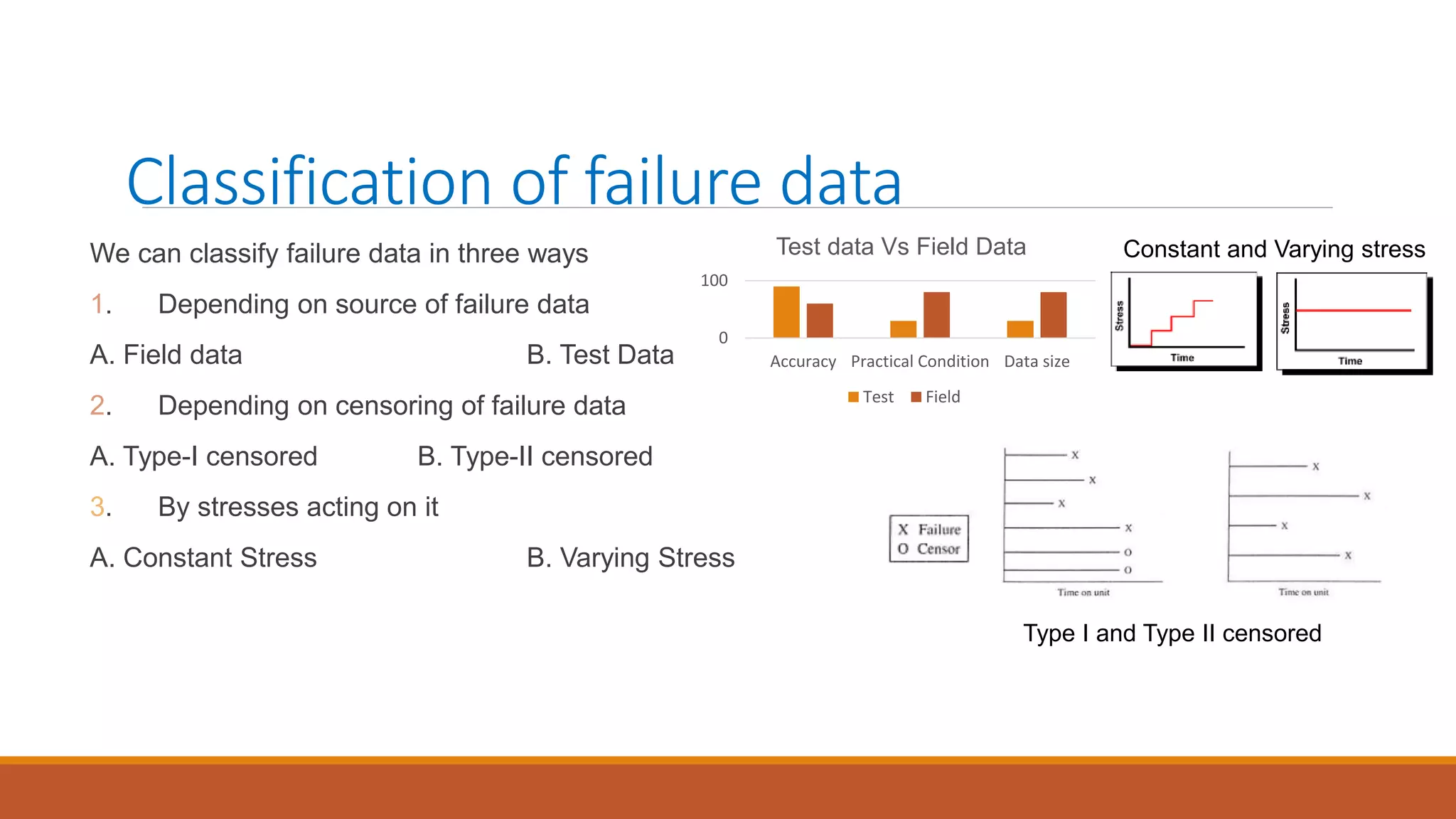
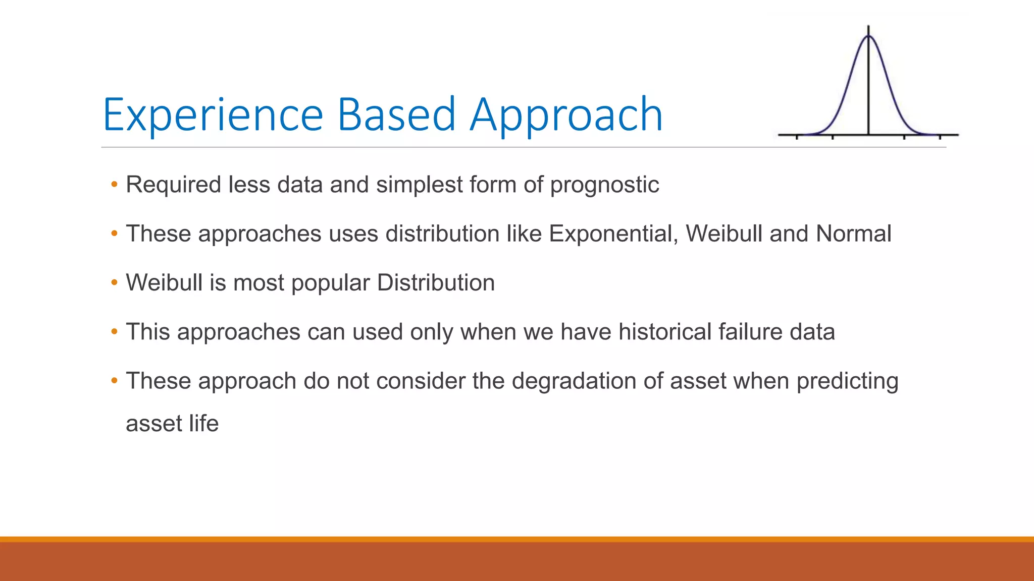
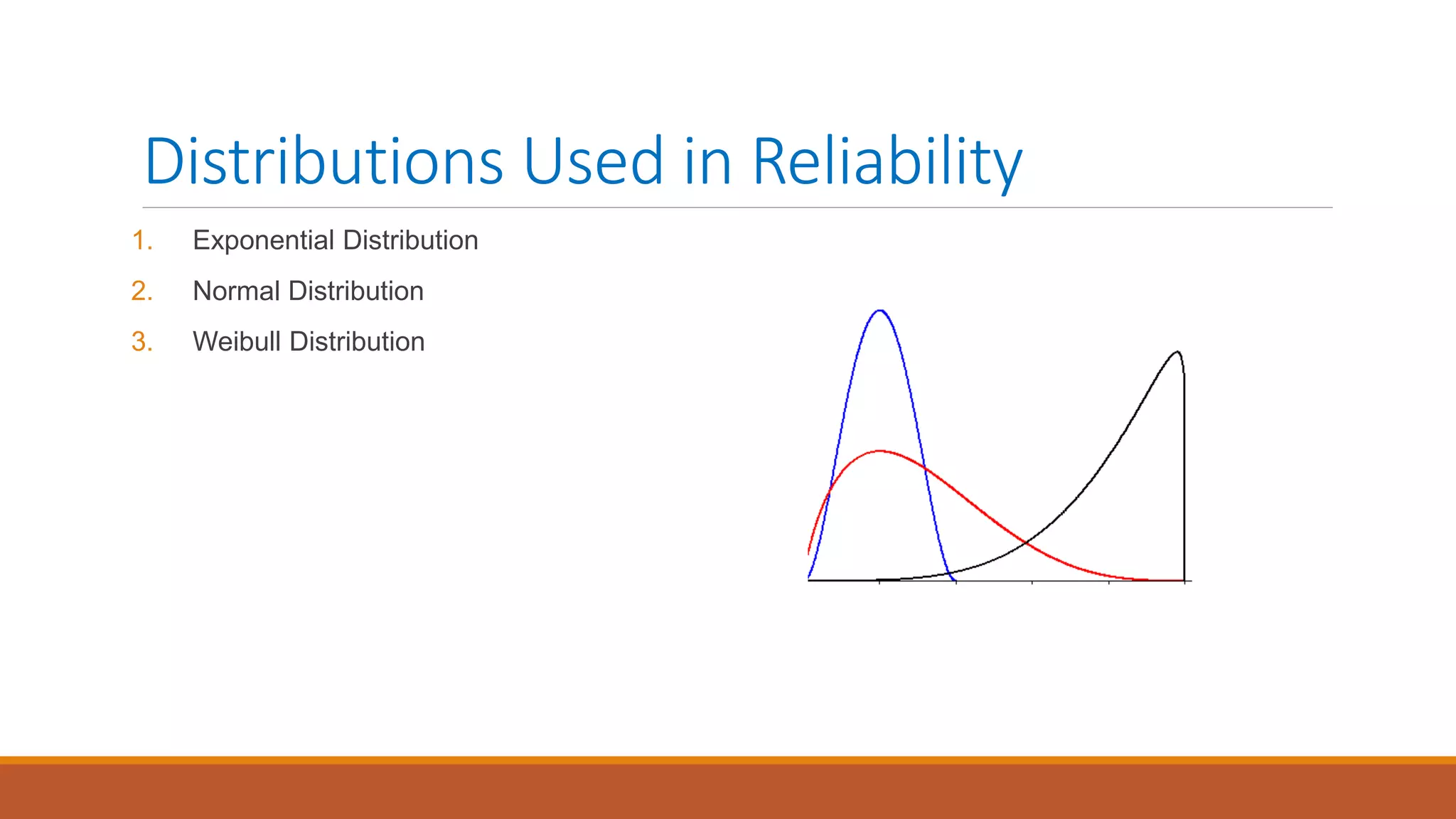
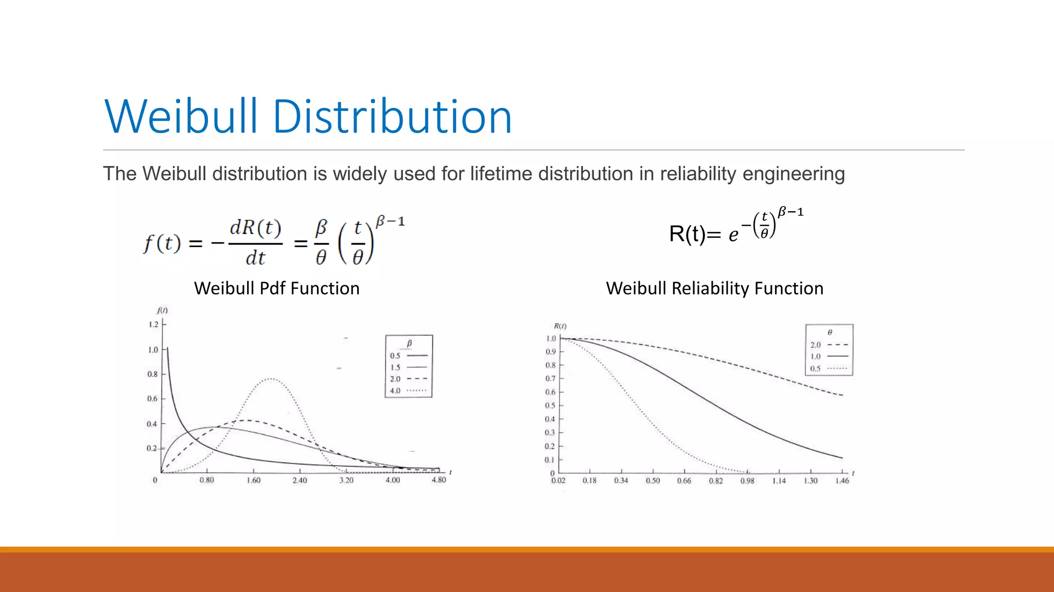
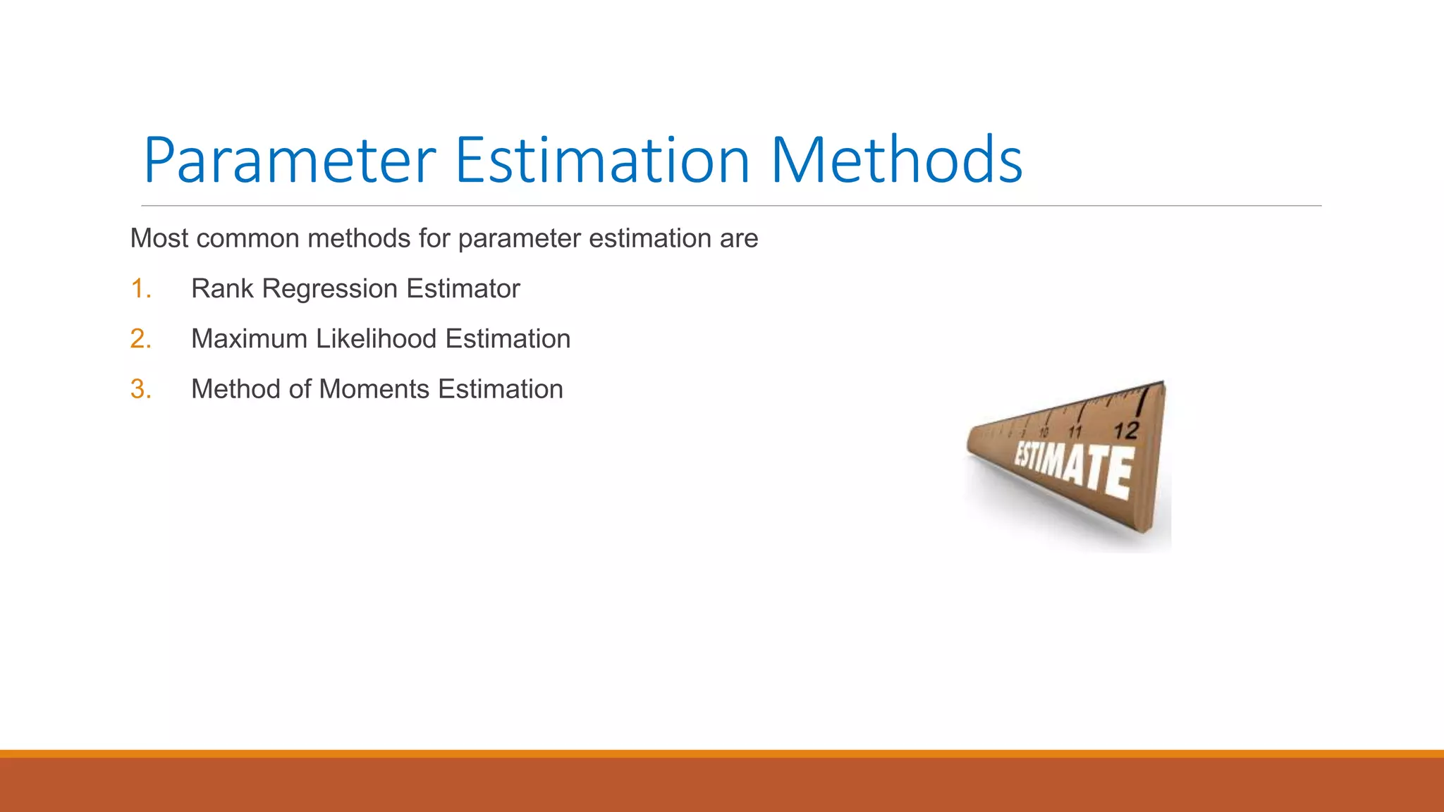
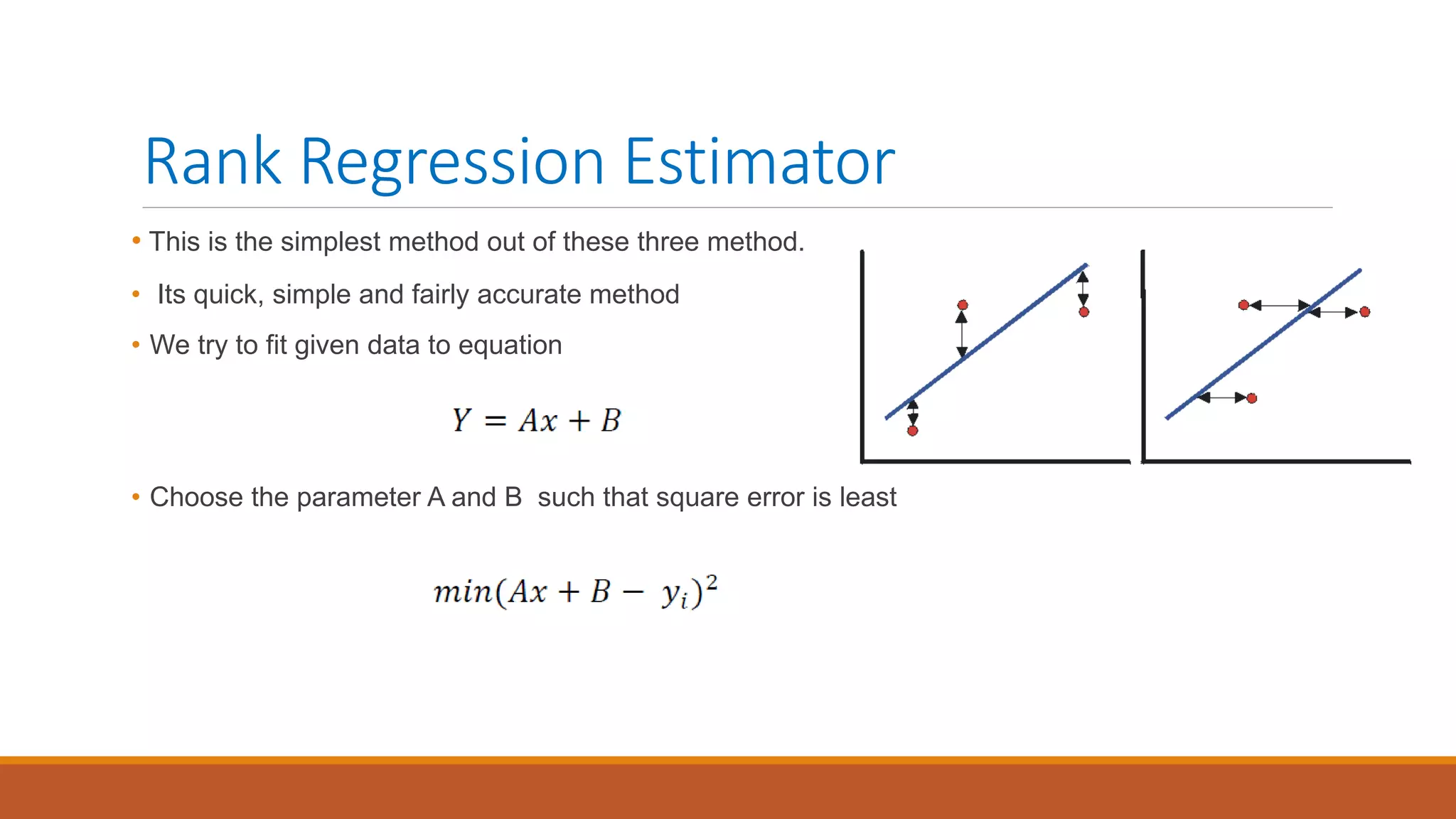
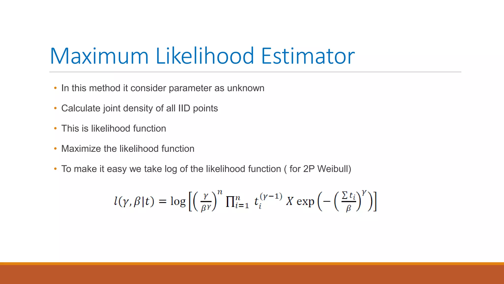
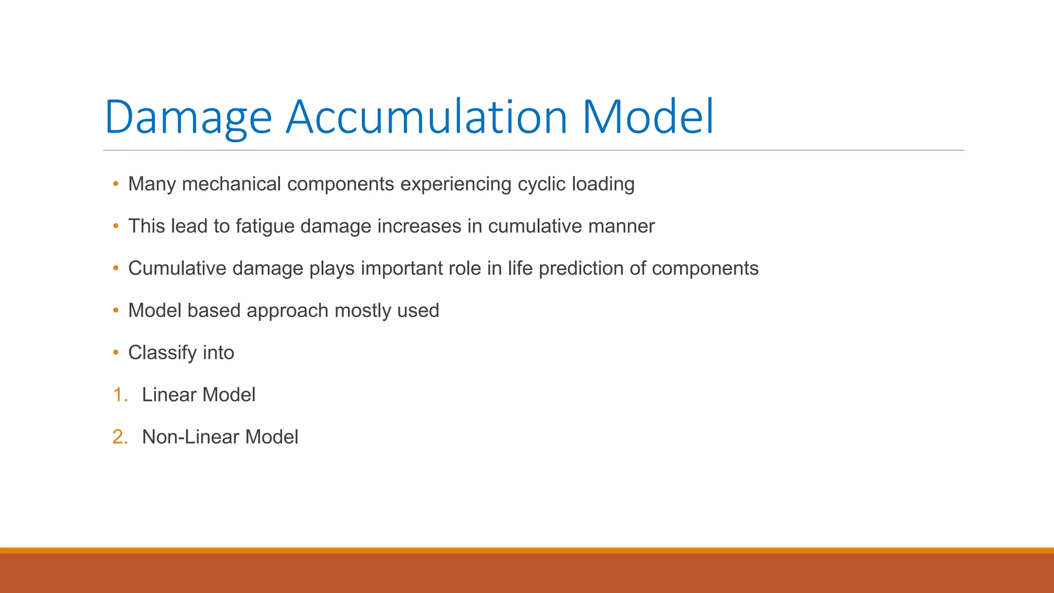
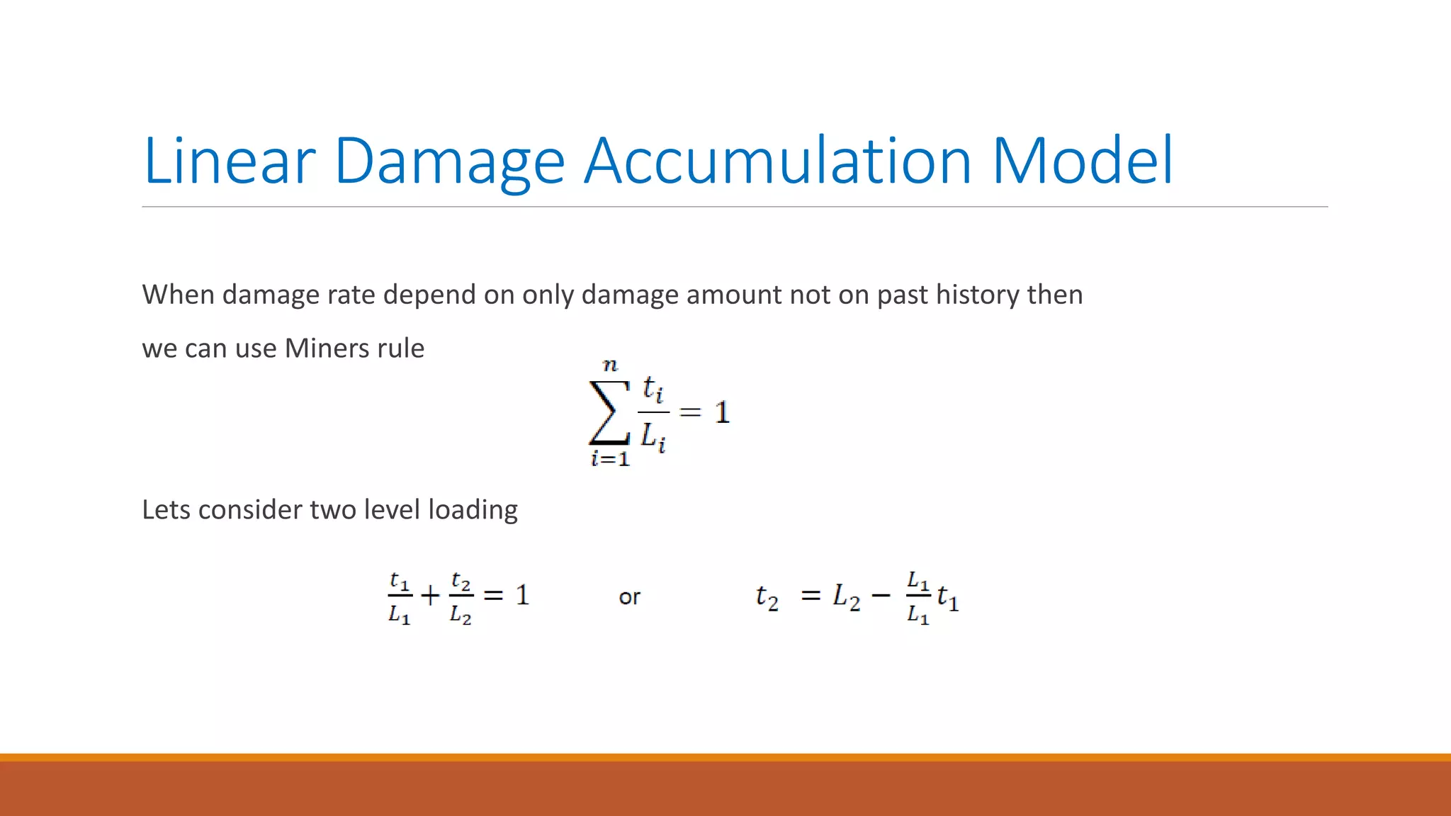
This document introduces nonlinear damage accumulation models. It discusses different types of failure data and prognostic approaches. Common life distributions like Weibull, exponential, and normal distributions are presented. Parameter estimation methods like maximum likelihood estimation and method of moments are described. Finally, linear and nonlinear damage accumulation models are covered, including the Manson-Halford and Huiying-Hong models which account for load interaction effects.

1. Introduction to Nonlinear
Damage Accumulation Model
Guided by Presented by
Prof. Asim Tewari Yogesh Nakhate
Prof. M.S. Kulkarni

2. Seminar Content
Introduction
Failure Data Types
Prognostic approaches
Life Distributions
Methods for Parameter Estimations
Damage Accumulation Model

3. Introduction
• Reliability
Reliability of is defined as probability of a system(component) will functional over a period of
time, can be expressed by
Or
Reliability is field of engineering which deals with life cycle management of a product
R(t)= 𝑃𝑟 𝑇 ≥ 𝑡

4. Reliability History
• Before World War II the term was linked mostly to repeatability
• In World War II, many reliability issues due to electronic equipment available at the time
• As aircraft and weapon equipment manufacturing production rate was increase exponentially
• Failure of these caused heavy loss in terms of human loss as well asset loss
• To get statistical study of failures reliability engineering becomes important
• Group form by US military AGREE (Advisory Group on the Reliability Electronics Equipment)
• Turning point for modern reliability.

5. Classification of failure data
We can classify failure data in three ways
1. Depending on source of failure data
A. Field data B. Test Data
2. Depending on censoring of failure data
A. Type-I censored B. Type-II censored
3. By stresses acting on it
A. Constant Stress B. Varying Stress
0
100
Accuracy Practical Condition Data size
Test data Vs Field Data
Test Field
Constant and Varying stress
Type I and Type II censored

6. Various prognostic approaches
In general approaches can be classified into four main group
1. Experienced based approach
2. Model based approach
3. Knowledge based approach
4. Data driven approach

7. Experience Based Approach
• Required less data and simplest form of prognostic
• These approaches uses distribution like Exponential, Weibull and Normal
• Weibull is most popular Distribution
• This approaches can used only when we have historical failure data
• These approach do not consider the degradation of asset when predicting
asset life

8. Model based approach
• This approach uses mathematics and dynamics
• Physics based models and statistical models are two kind of model based
approach.
• For example crack based model

9. Knowledge based approach
• In this approach human specialist are used to solve the problem
• This approach does not required any model as compare to model based
approach
• Expert systems and fuzzy logic systems are the two typical examples of
knowledge-based approaches

10. Data Driven Approach
• This approaches uses statistical and learning techniques which are used in
the theory of pattern recognition
• These Range from PCA, Neural Network, Decision trees, HMM
• Among them, Neural Networks and Hidden Markov Models are two typical
approaches, which are widely applied in prognostics

11. Distributions Used in Reliability
1. Exponential Distribution
2. Normal Distribution
3. Weibull Distribution

12. Exponential Distribution
The exponential distribution most commonly used in reliability engineering
Exponential Pdf Function Exponential Reliability Function
𝑓(𝑡) = 𝜆𝑒−𝜆𝑡

13. Normal Distribution
Normal distribution has been successful to model fatigue and wear out distribution
Phenomena
Normal Pdf Function Normal Reliability Function
R(t)
tt

14. Weibull Distribution
The Weibull distribution is widely used for lifetime distribution in reliability engineering
Weibull Pdf Function Weibull Reliability Function
R(t)= 𝑒
−
𝑡
𝜃
𝛽−1

15. Parameter Estimation Methods
Most common methods for parameter estimation are
1. Rank Regression Estimator
2. Maximum Likelihood Estimation
3. Method of Moments Estimation

16. Rank Regression Estimator
• This is the simplest method out of these three method.
• Its quick, simple and fairly accurate method
• We try to fit given data to equation
• Choose the parameter A and B such that square error is least

17. Maximum Likelihood Estimator
• In this method it consider parameter as unknown
• Calculate joint density of all IID points
• This is likelihood function
• Maximize the likelihood function
• To make it easy we take log of the likelihood function ( for 2P Weibull)

18. Method of Moment Estimator
• This is the one of the oldest method
• We calculate first and second moment of the sample using data points
• Then we generate the equation using parameters of the equations
• By two value of moment and two equations we estimate the parameters
• For two parameter Weibull

19. Damage Accumulation Model
• Many mechanical components experiencing cyclic loading
• This lead to fatigue damage increases in cumulative manner
• Cumulative damage plays important role in life prediction of components
• Model based approach mostly used
• Classify into
1. Linear Model
2. Non-Linear Model

20. Linear Damage Accumulation Model
When damage rate depend on only damage amount not on past history then
we can use Miners rule
Lets consider two level loading

21. Limitations of Linear Model
• In practical case model behaves differently than linear model
• The drawback for Miners rules that its independent on load conditions
• Its neglects load interaction effect
• To eliminate this drawback many fatigue module are proposed and many of them are nonlinear
• We will see model proposed by Manson & Halford

22. Non-linear Damage Accumulation Model
Non-linear fatigue damage accumulation model proposed by Manson and Halford
Where alpha can be calculated by

23. Non-linear Damage Accumulation Model
• Adjacent table shows Manson and Halford model result
• Experiment is conducted on crack propagation
of Mn45 steel
• Result is closed to experimental but still error
is measurable
• This is due to effect of load interaction
n1/
Nf1

24. Non-Linear model with load interaction
effect
Model is proposed by Huiying and Hong with load interaction effect, by changing the alpha
parameter
Where alpha can be calculated by

25. Non-Linear model with load interaction
effect
• Figure shows result of model proposed by Huiying
and Hong
• As explained in previous slide its consider effect of
load Interaction
• So considering load interaction reduces the error
• The proposed model, fatigue life prediction can be
obtained with high-precision

26. Conclusions
• Source of failure data can be either from field or from testing, field data is more realistic as its
comes from working environment of product while test data is more accurate and precise than
field data
• Censoring is the issue in reliability testing as component are removed before test is completed
• Weibull is the most commonly used distribution as it can have characteristics of other
distribution by setting shape and scale parameter
• Miners rule gives linear model for damage accumulation which is not in practical case
• Manson and Halford suggested non – linear model with exponential component in the equation
without load interaction effects
• Model suggested by Huiying and Huang considered load interaction so predict more accurate
results than Manson and Halford