Reliability and Safety

Welcome to Reliability and Safety
Training for project staff only.
Reliability and Safety (R&S)
Present By: Prakash Thapa
Head of process safety

Content
Module 1: Basic Elements in Reliability Engineering
Module 2: Interrelations of Reliability & Safety (R&S)
Module 3: The ideal R&S Process for Large Scale Systems
Module 4: Some Applications of R&S on LHC
Module 5: Lessons Learned from R&S Applications in various
Technologies

Module 1:
Basic Elements in Reliability Engineering
Content:
• Short R&S History
• Some Basic Terms
• A few Definitions and Formalisms
• From Components to Systems
• Important Methods
• Common Cause Failures
• Human Factor Issues
• Types of Uncertainties

Module 1:
Short History of R&S as Synonym of Risk
• Risk – very old Term (Perikles; 430 v.Chr)
“the worst thing is to rush into actions before the consequences have
been properly debated”, and “the Athenians are capable at the same
time of taking Risk and Estimating before-hand”
• „Trial and Error“ Approach (‘00 – ‘40)
• „Worst Case - Safety Case“ Studies (‘40 –)
• Recognition of Stochastic Events (‘40)
• Development of Reliability Theory (’40 -)
• Reliability Studies for Complex Systems (’50 -)
• Comprehensive Risk Studies (’70 -)
• Global Risk Management:
based on: Goal – Assignment – Proof (’90 -)
• „Risk Informed Decision Making“ (‘95 -)
• Risk Studies for Large Scale Test Facilities just in the
beginning (’00 - )
TimeAxis

Module 1:
Some Basic Terms
• Reliability:Reliability:
The ability of an item to operate under designated operating
conditions for a designated period of time or number of
cycles.
Remark: The ability of an item can be designated through a
probability, or can be designated deterministic
• Availability:Availability:
The probability that an item will be operational at a given time
Remark: Mathematically the Availability of an item is a
measure of the fraction of time that the item is in operating
conditions in relation to total or calendar time
R&S Training Course
CERN, February 2002

Module 1:
Some Basic Terms
• Maintainability:Maintainability:
The probability that a given active maintenance action, for an
item under given conditions of use can be carried out within a
stated time interval when the maintenance is performed under
stated conditions and using stated procedures and resources
(IEC 60050)1)
Remark: probabilistic definition
• Safety:Safety:
Freedom from unacceptable risk of harm
Remark: very vague definition
• RAMS:RAMS: An acronym meaning a combination of Reliability,
Availability, Maintainability and Safety

Module 1:
Some Basic Terms
Dependability
Reliability
Safety
Availability
Maintainability
Today‘s Understanding for PuristsToday‘s Understanding for Purists

Module 1:
Some Basic Terms
• Hazard:Hazard: A physical situation with a potential for
human injury, damage to property, damage to the
environment or some combination of these
• Individual Risk:Individual Risk: The frequency at which an
individual may be expected to sustain a given level
of harm from the realisation of specified hazards
• Social Risk:Social Risk: The frequency with which a specified
number of people in a given population, or
population as a whole, sustain a specified level of
harm from the realisation of specified hazards

Module 1:
A few Definitions and Formalisms
For non-repaired items the reliability function:
t ∞
R(t) = exp [ - ∫ λ(x)dx] = ∫ f(x)dx
0 t
where
λ(x) is the instantaneous failure rate of an item
f(x) is the probability density function of the time to failure of the item
when λ(t) = λ = constant, i.e. when the (operating) time to failure is exponentially
distributed
R(t) = exp(-λt)
Example:
For an item with a constant failure rate of one occurrence per operating year and a
required time of operation of six month, the reliability is given by
R(6m) = exp(- 1 x 6/12) = 0,6065

Module 1:
Failure RateFailure Rate λλ follows normallyfollows normally
the so-called “bath tube curve”the so-called “bath tube curve”
Time
Utilisation
Phase
Constant Failure Rate
Debugging Wearout
λ

Module 1:
Failure RateFailure Rate λλ are often published in Date Booksare often published in Date Books
A few ExamplesA few Examples
• Offshore Reliability Data; OREDA Handbook; 2nd
Edition; distributed by
Det Norska Veritas Industri Norge AS; DNV Technica 1992
ISBN 82 515 0188 1
• Handbook of Reliability Data for Electronic Components; RDF 93
English Issue 1993; Copyright France Telecom – CNET 1993
• Reliability Data of Components in Nordic Nuclear Power Plants; T-book
3rd
Edition; Vattenfall AB; ISBN 91-7186-294-3
• EUREDATA; Published by Joint Research Centre (JRC) Ispra, It
• Links for Data Informations see at ESRA Homepage

Module 1:
For non-repaired items:For non-repaired items:
If observed failure data are available for n non-repaired items with constant failure
rate, then the estimated value of λ is given by
n
λ = n / Σ TTFi
i=1
where TTFi is time to failure of item i
Example:
For 10 non-repaired items with a constant failure rate, the observed total operating
time to failures of all the items is 2 years. Hence
λ = 10/2 = 5 failures per year

Module 1:
For non-repaired items:For non-repaired items:
∞
MTTF = ∫ R(t)dt ………Mean Time To Failure
0
When time to failure is exponentially distributed,
MTTF = 1 / λ
Example:
For a non-repaired items with a constant failure rate of two failures per four
years of operating time,
MTTF = 1 / 2 / 4 = 2 years = 17.520 h

Module 1:
For repaired items with zero time to restoration the reliability function is givenFor repaired items with zero time to restoration the reliability function is given
t1
R(t1,t2) = R(t2) + ∫ R(t2 – t) ⋅ z(t)dt
0
where
R(t2), represents the probability of survival to time t2, and
the second term represents the probability of failing at time t(t< t1) and, after
immediately restoration, surviving to time t2
z(t) is the instantaneous failure intensity (renewal density) of the item, i.e. z(t)dt is
approximately the (unconditional) probability that a failure of the item occurs during
(t, t + ∆t)
Example:
For a repaired items with a constant failure rate of one failures per operating year
and a required time of operation without failure of six months, the reliability is given
by
R(t, t + 6) = exp (-1 x 6/12) = 0,6065

Module 1:
For repaired items with zero time to restoration the Mean Time To Failure isFor repaired items with zero time to restoration the Mean Time To Failure is
givengiven
∧ ∞
MTTF = ∫ R(t)dt
0
When observed operating time to failures of n items are available, then an
estimate of MTTF is given by
∧
MTTF = total operating time / kF
Example:
For a repaired items with a constant failure rate of 0,5 failures per year
MTTF = 1/0,5/1 = 2 years = 17.520 h

Module 1:
Consider:Consider:
If a repaired item with zero time to restoration operates continuously, and if
the times to failure are exponentially distributed three often used terms are
equal
MTTF = MTBF = MUT = 1/λ
MTTF Mean Time To Failure
MTBF Mean Time between Failure
MUT Mean Uptime

Module 1:
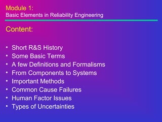
Repaired items with non-zero time to restorationRepaired items with non-zero time to restoration
The reliability of a repaired item with non-zero time to restoration for the
time interval(t1, t2) may be written as
t1
R(t1, t2) = R(t2) + ∫ R(t2 – t)ν(t)dt
0
where the first term R(t2) represents the probability of survival to time t2, and
the second term represents the probability of restoration (after a failure) at
time t(t < t1), and surviving to time t2
ν(t) is the instantaneous restoration intensity of the item
When the times to failure are exponentially distributed, then
R(t1, t2) = A(t1)exp(-λ ⋅ (t2 – t1))
where A(t1) is the instantaneous availability at time t1, and
lim R(t, t + x) = [MTTF / (MTTF + MTTR)] exp(-λt)
t →∞

Module 1:
When times to failure and times to restoration are exponentially distributed, then,
using either Markov techniques or the Laplace transformation, the following
expression is obtained:
R(t1, t2) = (µR/(λ + µR) + λ/(λ + µR)exp[-(λ + µR) t1]exp[-λ ⋅ (t1 – t2)]
and
lim R(t, t + x) = µR /(λ + µR) exp(-λx)
t → ∞
Example:
For a item with λ = 2 failures per operating year and a restoration rate of µR = 10
restorations per (restoration) year, and x = 1/4
lim R(t, t + 1/4) = 10/12 exp(-2 x 1/4) = 0,505
t → ∞

Module 1:
_
We can define a asymptotic mean availability A of an item
_ _
A = lim A (t1, t2) = A = MUT / (MUT + MTTR)
t2 → ∞
where
MTTR… Mean Time to Repair
Example:
For a continuously operating item with a failure rate of λ = 2 failures per operating
year and a restoration rate of µR = 10 restorations per year
then
_
A = (0, ¼) = 10/12 + 2/144 {[(exp(-12 x 0) – exp(-12 x ¼)] / ¼ - 0} = 0,886
= (0, 1) = 0,833

Module 1:
Additional Formulas see e.g. in the following TextbooksAdditional Formulas see e.g. in the following Textbooks
(random sample of useful books)(random sample of useful books)
• Birolini, A., Quality and Reliability of Technical Systems; Springer 1997
2nd
Edition; ISBN 3-540-63310-3
• Hoyland A., & Rausand, M., System Reliability Theory; John Wiley &
Sons; 1994; ISBN 0-471-59397-4
• Modarres, M., Reliability and Risk Analysis; Marcel Dekker, Inc. NY;
1993, ISBN 0-8247-8958-X
• Schrüfer, E., Zuverlässigkeit von Meß- und Automatisierungseinrich-
tungen; Hanser Verlag, 1984, ISBN 3-446-14190-1
• Knezevic, J., Systems Maintainability, Chapman & Hall, 1997,
ISBN 0 412 80270 8
• Lipschutz, S., Probability, Schaums Outline Series, McGraw-Hill Book
Company, 1965, ISBN 07-037982-3
• IEC 61703, Ed 1: Mathematical Expressions for Reliability, Availability,
Maintainability and Maintenance Support Terms, 1999
http://www.dke.de

Module 1:
Types of MaintenanceTypes of Maintenance
Maintenance
Corrective
Maintenance
Preventive
Maintenance
Condition
dependant
Reliability
centred
Intersection of Theory und Practice
Time
dependant

Module 1:
Maintainability MeasuresMaintainability Measures
Probability of Task Completion:
PTCDMT = P(DMT ≤ Tst) = ∫
0
Tst
m(t)dt
Tst ….stated time for task completion
m(t)…probability density function of DMT
Mean Duration of Maintenance Task:
MDMT = E(DMT) = ∫
0
∞
t x m(t)dt
E(DMT)… expectation of the random variable DMT

Module 1:
Maintenance and the Exponential DistributionMaintenance and the Exponential Distribution
m(t) = (1 / Am ) · exp – (t / Am) , t > 0
In case of exponential probability distribution:
m(t) = P(DMT ≤ t) = 1 – exp – (t / Am)
DMT….Duration of Maintenance Task
Am…….Scale parameter of the exp. distribution = MDMT
Example:
On average it takes 10 days to restore a specific machine; find
the chance that less than 5 days will be enough to successfully
complete the restoration:
Solution:
m(t) = (1/10) · exp - (t / 10)
and P(DMT) ≤ 5 = M(5) = 1 - exp – 5/10 = 1 - 0,61 = 0,39

Module 1:
From Components to Systems
We have to recall some Basic Laws of ProbabilityWe have to recall some Basic Laws of Probability
A and B are mutually exclusive events than the probability that either of them occurs
in a single trial is the sum of their probability
Pr{A + B} = Pr{A} + Pr{B}
If two events A and B are general, the probability that at least one of them occurs is:
Pr{A + B} = Pr{A} + Pr{B} – Pr{AB}
Two events, A & B, are statistically independent if and only if
Pr{AB} = Pr{A} ⋅ Pr{B}
Bayes Theorem
Pr{AiB} = PR{Ai} ⋅ Pr{BAi} / [ Σi Pr{BAi} ⋅ Pr{Ai}]
More see in e. g. Schaum’s Outline Series [Seymour Lipschutz]:
“Theory and Problems of Probability”, McGRAW-HILL Book Company

Module 1:
We know
R(t) = e – λ .t
= 1 – Q(t)
Q(t) = 1 – R(t) Qav ~ λ . t / 2
λ = 1 / MTBF [h-1
]
MTBF = Operational Time / Number of Stops
MTTR = Sum of Repair Time / Number of Repairs
For the System we yield:
λS = Σ λ = 0,0125 + 0,0125 = 0,025 1/h
MTBFS = 1/(1/MTBF + 1/MTBF) =1/(1/80 + 1/80) = 40 h
RS = R x R = 0,9 x 0,9 = 0,81
QS = Q + Q – (Q x Q) = 0,1 + 0,1 – 0,01 = 0,19 = 1 - 0,81
Serial SystemSerial System
MTBF = 80
λ = 1/80 = 0,0125
R = 0,9
MTBF = 80
λ = 1/80 = 0,0125
R = 0,9
RS = Ri
n

Module 1:
We know
R(t) = e – λ . t
= 1 – Q(t)
Q(t) = 1 – R(t) Qav ~ λ . t / 2
λ = 1 / MTBF [h-1
]
MTBF = Operational Time / Number of Stops
MTTR = Sum of Repair Time / Number of Repairs
MTBF = 80
λ = 1/80 = 0,0125
R = 0,9
MTBF = 80
λ = 1/80 = 0,0125
R = 0,9
Parallel SystemParallel System
For the System we yield
λS = 2 λ / 3 = 0,0083 1/h
MTBFS = 80 + 80 – 1/(1/80 + 1/80) = 120 h
RS = 1 - [(1 - R) x (1 - R)] = 1 – (1 - 0,9) x (1 – 0,9) = 0,99
RS = R + R – R x R = 0,9 + 0,9 – 0,9 x 0,9 = 0,99
QS = Q x Q = 0,1 x 0,1 = 0,01
RS = 1 - (1 - Ri)n

Module 1:
Mixed SystemMixed System
0,95
0,99
0,98
0,90
0,99 0,97
For the System we yield
RS = 1– [(1– 0,95)(1– 0,99)] x 0,98 x {1– [(1– 0,99) x 0,97 x (1- 0,90)]}
= 0,9995 x 0.98 x 0,99603
RS = 0,97562 ~ 0,97
The Unreliability
QS = 1 – R = 0,02438 ~ 0,03

Module 1:
Nowadays we calculate Reliability Characteristics byNowadays we calculate Reliability Characteristics by
the means of commercial PC programs like:the means of commercial PC programs like:
• Cafta (USA)
• Care (Israel)
• Item Software (UK)
• Isograph (UK)
• Relex (USA)
• Risk Spectrum (S)
• Saphire (USA)
For further information look for Software presentations at
ESREL Conference Sites, e.g. ESREL99; ESREL2001,
ESREL2002

Module 1:
Important Methods
Failure Mode
of
Item
Cause Effect
Mode
1 - n
Nowadays
a Semi Quantitative
Procedure using a
three parameter
grading system
RPZ
FMEA Principle:FMEA Principle:
it represents a qualitative structure
“what” can be happen “why”

Module 1:
Important Methods
Ventilator
blocked
large FTs
consist of 5.000
Function Elements
Fault Tree Principle:Fault Tree Principle:
A qualitative structure
“how” the system fails
Using Failure Rates
we can perform
the Fault Tree quantification
Cooling
fails
Motor
do not start
Switch
do not close
“or”
“or”
No Impulse

Module 1:
Important Methods
D E
or
TOP Event
TE = A + BD + BE + CD + CE
B + C D + E
and
B C
or
SimplifiedSimplified
Cut Set ExampleCut Set Example
IF A, B, C, D, E = O,1 than TE = 0,045
BD+BE+CD+CE A
or

Module 1:
Important Methods
Large Event Trees
consist of dozen‘s
of branches
Event Tree Principle:Event Tree Principle:
it represents a
qualitative structure
“what” can be happen
Using Probabilities
we can perform the
Event Tree Quantification
Event Sequence
Condition ESk1
Event Sequence
Condition ESk2
Plant Damage
State, PDSj
p (no)
p (yes)Initiating Event
IEi
e.g. Cooling Pipe Break

Module 1:
Important Methods
Pump
d.n.st.
Valve
d.n.op.
IEs
Initating Events
1 - i
System Functions 1 - j
Fault Trees 1 - k
Consequence:
Type
Frequency
Amount
Basic Events
Function
Failure
PSA ModelPSA Model
An Integrative Model
of Event Trees
and Fault Trees
Large PSA Models
consist of a fifty
Event Trees and
a hundred of Fault Trees
OR

Module 1:
Important Methods
Markov Modelling / ChainsMarkov Modelling / Chains
Three Types:
• Homogeneous Continuous Time Markov Chain
• Non-Homogeneous Continuous Time Markov Chain
• Semi-Markov Models
Pros
- very flexible capability
- good for repair
- good for standby spares
- good for sequence dependencies
- Good for different type of fault coverage, error handling and recovery
Cons
- can require large number of states
- modelling is relative complex model often different from physical or
logical organisation of the system

Module 1:
Important Methods
Markov Modelling / ChainsMarkov Modelling / Chains
Simple Example
• Control System
• Two processors; 1 active, 1 hot backup
• Fault coverage may be imperfect
• c = pr {fault detected and recovery is successful given
processor fault occurs}
• 1 – c = pr {fault is not detected or recovery is unsuccessful
given processor fault occurs}
• λ = Failure Rate
• µ = Repair Rate
1
F
2
λ
µ
2cλ
2(1-c)λ

Module 1:
Important Methods
Stress Strength
Safety Factor
N/mm²
pdf
Structural ReliabilityStructural Reliability
(simplified one dimensional case)
a measure for probability of failure

Module 1:
Common Cause Failures
Type of Failures of ItemsType of Failures of Items
Random
Failures
Dependant
Failures
Consecutive
Failures
Failures
of identical
Items
Functional
Failures
Failure
of a few
Items
Environm.
caused
Failures
Design
Failures
One has to model
these different types !

Module 1:
The Boolean representation of a three component
system considering Common Cause Failures (CCF)
shows as following:
AT = Ai + CAB + CAC + CABC
AT….total failure of component A
Ai…..failure of component A from independent causes
CAB..failure of component A and B (and not C) from common
cause
CAC..equivalent

Module 1:
The simple single parameter model called
β factor model looks like
Qm = β . Qt
β= e.g. 0,1 that means in other words
10% of the unavailability of a system would be
caused by common cause failures
Some other models are shown in the next copy

Module 1:

Module 1:
Human Factor Issues
Human Factor Issues are massive involved in theHuman Factor Issues are massive involved in the
R&S TechnologyR&S Technology
• Human Operator Reliability in control rooms
• Human Reliability in maintenance work
• Human Reliability in abnormal, accidental and emergency
conditions
• Man – Machine Effectiveness
• Human Operators in control loop systems
• Ergonomics for control, supervision and maintenance of
systems

Module 1:
Human Factor Issues
HR Models of the first generationHR Models of the first generation
• THERP (Techniques for Human Error Program)
• HCR (Human Cognitive Reliability Model)
• PHRA (Probabilistic Human Reliability Analysis)
• SLIM (Success Likelihood Index Method)
Within THERP the so called HRA Action Tree represents the
procedure used for estimating probabilities
Ptot =
A + (a×B)
+ (a×b×C×D)
+ (a×b×C×d×E)
+(a×b×c×E)
Failure
Success

Module 1:
Human Factor Issues
HR Models of the second generationHR Models of the second generation
• ATHENA (NRC)
• CREAM (Halden)
• MERMOS (EDF)
• FACE (VTT)
and many others. These models are more cognitive oriented
as the first generation models
The challenge nowadays is the estimation of HEPs for “Errors
of Commission”
For “Errors of Omission” a soundly based tool box and
validated data are available

Module 1:
Software Issues
Why Software Reliability Prediction (SRP) is needed?
• Amount & Importance of software is increasing
• Software accounts for approximately 80 % of switch failures
• Software reliability is not improving fast
• Software is costly to fix
• Motivation, pressure and number of experts for doing SRP
is limited
Basic Questions in SRP:
• At what rate do failures occur ?
• What is the impact of these failures ?
• When will faults be corrected ?

Module 1:
Software Issues
Important DefinitionImportant Definition
FailureFailure…. An event in which the execution of a
software system produces behaviour which
does not meet costumer expectation
(functional performance)
FaultFault……The part of the software system which must
be repaired to prevent a failure.

Module 1:
Software Issues
If we have an observed data example we can calculateIf we have an observed data example we can calculate
λλ(t) (failure intensity/rate)(t) (failure intensity/rate)
if a Logarithmic Poisson Distribution is suitable:
λ(t) = a / (b · t + 1)
The parameters to be estimated are a and b
For that we need the likelihood function or
the probability that the observed data occur:
L(data) = Πj Pr{yj failure in period j}

Module 1:
Software Issues
Example:Example:
Period j System Month tj Number of Failures yj
1 23 55
2 52 62
3 89 47
4 137 52
5 199 56
6 279 42
7 380 47
8 511 49

Module 1:
Software Issues
Example:Example:
Parameter estimates: a = 2,93; b = 0,016
λ(t) = 2,93 / (0,016 · t + 1)
Thus:
Estimates of failure intensity at 1.000 system month:
λ(t) = 2,93 / (0,016 x 1000 + 1) = 0,17 failures per system month
Estimate the mean cumulative number of failures at 5.000
system month:
2,93 / 0,016) · ln (0,016 · t +1) =
2,93 / 0,016) · ln (0,016 x 5.000 +1) = 805 failures
Today’s References [IEC 61508; Belcore Publications plus Handout]

Module 1:
Types of Uncertainties
Within the process of R&S we have to be awareWithin the process of R&S we have to be aware
about - at least - three type of uncertaintiesabout - at least - three type of uncertainties
• Parameter uncertainties (aleatory uncertainties)
• Model uncertainties (epistemic uncertainties)
• Degree of completeness
Problems and unresolved issues performing an uncertainty
assessment increases as this sequence
But
“some information about uncertainties is better than nothing”

Module 1:
Some Standards
IEC 300 Dependability Management
IEC 605 Equipment Reliability Testing
IEC 706 Guide to the Maintainability of Equipments
IEC 50(191) Procedure for Failure Mode and Effect Analysis (FMEA)
IEC 1014 Programmes for Reliability Growth
IEC 1025 Fault Tree Analysis (FTA)
IEC 1070 Compliance Test Procedure for Steady State Availability
IEC 1078 Reliability Block Diagrams
IEC 1123 Reliability Testing
IEC 1160 Formal Design Review
IEC 1146 Reliability Growth Models and Estimation Methods
IEC 1165 Application of Markov Methods
IEC 61508 Functional safety of electrical/electronic/programmable
electronic safety related systems
Others for Reliability Issues: CENELEC, IEEE, ISO, MIL, ASME, etc.

Module 2:
Systems Reliability towards Risk Informed Approach
Content:Content:
• Systems Reliability towards Risk Informed Approach
• Anatomy of Risk
• Some Definitions
• Living Models
• Reliability Growth Management
• Risk Monitoring
• How Safe is Safe Enough?

Module 2:
Living
Process
(modern)
Plant Model
Historical
Experience
Trial and Error
(past)
Future
Behaviour

Module 2:
Deterministic in System ReliabilityDeterministic in System Reliability
– Design Process:
based on pre-defined rules and criterions derived from
experiences
– Calculation Process:
based on determined laws and formulas, calculating
point values
– Review Process:
check of the compliance with rules and standards
– Decision Making Process:
yes / no - go / no go answers based on rule compliance

Module 2:
Probabilistic in System ReliabilityProbabilistic in System Reliability
– Design Process:
based on pre-defined rules and criterions based on
experiences
plus probabilistic goals and targets
– Calculation Process:
based on determined laws and formulas plus
uncertainties and random variables, calculating
distribution functions
– Review Process:
check of the compliance with rules and standards
plus check of the compliance with the goals and targets
– Decision Making Process:
yes / no - go / no go answers based on risk insights

• In the Deterministic Approach we use formalisms derived
from best practice and fitted with single point values as a first
guess
• The „Real World“ do not follow that formalisms based on
single point values. Practical all values required show
spreads (uncertainties) and / or a stochastic behaviour
Therefore exists a challenge for modernTherefore exists a challenge for modern
analysis techniques and numerical solutionsanalysis techniques and numerical solutions
(e.g. Simulations)(e.g. Simulations)
I advocate for the extension from deterministicI advocate for the extension from deterministic
approach towards probabilistic models to considerapproach towards probabilistic models to consider
the stochastic behaviour and the uncertaintiesthe stochastic behaviour and the uncertainties
Module 2:

Module 2:
Probabilistic towards Risk Informed ApproachProbabilistic towards Risk Informed Approach
PROS
– it is an extension of the deterministic basis
– it is supported quantitatively by historical experiences
– it models determined, random and uncertain elements
– it is quantitative and therefore appropriate for sensitivity, importance
and optimisation studies
– it integrates design, manufacturing and operational aspects
– it integrates various safety issues and allows rankings
– it shows explicit vagueness and uncertainties
CONS
– relatively new, more complex, and not well understood
– larger projects, harder to get financial support
– harder transformation of results into “yes or no” decisions

Module 2:
Causes
BasicEvents
Fault Tree
Consequences
Event Tree
„Bow – Tie“ Logic
Initiating
Event
Fault Tree
Basis Events

Module 2:
System
and
Reliability
Analysis
Identification of IEs
Database Generation
Common Cause Analysis
Human Factor Analysis
Fault Tree Analysis
System Response Analysis
Event Tree Analysis
LHC
Plant Damage States
and their Frequencies
Systems Reliability
Characteristics

Module 2:
Anatomy of Risk
Risk of a Plant
Type, Amount and Frequency of Consequences
Consequences Frequencies
Release
Parameter
Receptor
Parameter
IEs
Frequencies
Conditional
Probabilities
Classical
Decomposition

Module 2:
Some Definitions
Reliability Insights generated by Importance MeasuresReliability Insights generated by Importance Measures
• Fussel-Vesely = [PR{top} – Pr{topA = 0}] / Pr{top}
Weighted fraction of cut sets that contain the basic event
• Birnbaum = Pr{topA = 1} – Pr{topA = 0}
Maximum increase in risk Associated with component A is
failed to component A is perfect
• Risk Achievement worth = Pr{topA = 1} / Pr{top}
The factor by which the top probability (or risk) would
increase if component A is not available (not installed)
• Risk Reduction Worth = Pr{top} / Pr{topA = 0}
The factor by which the risk would be reduced if the
component A were made perfect

Module 2:
Living Models
In R&S we have to learn permanently from the past; thatIn R&S we have to learn permanently from the past; that
means it is an ongoing, never ending process, we call itmeans it is an ongoing, never ending process, we call it
Living ProcessLiving Process
It is strongly recommended to establish and the store all the
models and data with the means of computerised tools
This helps to manage in a more efficient way three important
issues
• System Changes
• Personal Changes
• Increasing State of Knowledge

Module 2:
Reliability Growth Management
Basic Structure
• Management
• Testing
• Failure Reporting, Analysis and Corrective Action System
(FRACAS)
During Test we observe
• Type A modes (not fixed)
• Type B modes (fixed)
At beginning of the test operation
λi = λA + λB
Effectiveness Factor EF
λinh = λA + (1 - EF) λA
(more details for growth models see MIL-HDBK-189)

Module 2:
Risk Monitoring
Statistical
Data
System
Information
PSA
Modell
Current
Situation
Reliability
Information
„What
Happens If“

Module 2:
Risk Monitoring
Operational TimeOperational Time
ReliabilityReliability
CharacteristicCharacteristic
AbnormalAbnormal
EventEvent ReliningRelining
Unknown LevelUnknown Level
without calculationwithout calculation
Base LineBase Line
„„Risk Profil“Risk Profil“
of a plantof a plant

Module 2:
How Safe is Safe Enough?
Typical way of ThinkingTypical way of Thinking
BroadlyBroadly
AcceptableAcceptable
IntolerableIntolerable
ALARPALARP
Risk unjustifiable
Tolerable only
if reduction impracticable
or cost grossly
disproportionate
Tolerable if cost
of reduction exceeds
improvement
Maintain assurance
that risk is at this level
Benchmark

Module 2:
List of important qualitative Risk CharacteristicsList of important qualitative Risk Characteristics
related to Tolerabilityrelated to Tolerability ofof RiskRisk
Qualitative Characteristics Direction of Influence
Personal Control Increase Risk Tolerance
Institutional Control Depends on Confidence
Voluntariness Increase Risk Tolerance
Familiarity Increase Risk Tolerance
Dread Decrease Risk Tolerance
Inequitable Distribution Depends on Individual Utility
Artificiality of Risk Source Amplifies Risk Awareness
Blame Increase Quest for Social
and Political Response

Module 2:
Z The Netherlands
(new establishments)
Z Canada Z UK
1 IR < 10-6
Housing, schools,
hospitals allowed
i IR < 10-6
Every activity
allowed
A PED < 10-6
Insignificant risk
area
2 10-6
< IR < 10-5
Offices, stores,
restaurants allowed
ii 10-6
< IR < 10-5
Commercial activity
only
B 10-6
< PED < 10-5
Risk assessment
required
3 IR > 10-5
Only by exemption
iii 10-5
< IR < 10-4
Only adjacent
activity
C PED > 10-5
High risk area
iv IR > 10-4
Forbidden area
Risk Contours in Land Use Planning (z-Zone)Risk Contours in Land Use Planning (z-Zone) [Okstad; ESREL01][Okstad; ESREL01]

Module 2:
11 1010 100100 100010000,10,1
Type of ExposureType of Exposure
Cancer
Pneumonia
Mining
Suicide
Motorcar traffic
Industrial work
Chemical industry work
Electrical current
Lightning
Individual Risk (D)Individual Risk (D)
number per mio persons and yearnumber per mio persons and year

Module 3:
The ideal R&M Process for Large Scale Sys
Content:
• The ideal Process
• Anatomy of Risk
• From R&S Goals via the Implementation into the System to
the Proof of the Compliance
• Constrains and Problems Implementing an ideal Process

Module 3:
The ideal Process
The ideal R&S process consists (simplified) ofThe ideal R&S process consists (simplified) of
four main elements:four main elements:
• Establishment of the Risk Policy
• Evaluation and Assessment of the Risk Concerns
• Performing Risk Control
• To do Decision Making
The process is highly intermeshed and iterative!The process is highly intermeshed and iterative!
and multi-disciplinaryand multi-disciplinary

Module 3:
The ideal Process
• To make this ideal process useful for application we need
quantitative Safety Risk / Goal witch is tolerable by the
society.
• There is trend to use as orientation for this Goal the so
called Minimal Endogen Mortality (MEM Value) which is the
individual risk for young people to die per year
• This MEM value is given in most of the countries at al level of
2 x 10-4
per person year
• Based on this number some experts advocate for a Global
Individual Risk Goal for Hazardous Installations at a level of
10-5
per person year.

Module 3:
The ideal Process
List of important qualitative Risk CharacteristicsList of important qualitative Risk Characteristics
related to the Tolerabilityrelated to the Tolerability ofof RiskRisk
Qualitative Characteristics Direction of Influence
Personal Control Increase Risk Tolerance
Institutional Control Depends on Confidence
Voluntaries Increase Risk Tolerance
Familiarity Increase Risk Tolerance
Dread Decrease Risk Tolerance
Inequitable Distribution Depends on Individual Utility
Artificiality of Risk Source Amplifies Risk Awareness
Blame Increase Quest for Social
and Political Response

Module 3:
The ideal Process
The ideal process integrates design, construction, andThe ideal process integrates design, construction, and
operational parameters from the system, the operatoroperational parameters from the system, the operator
and the environment.and the environment.
The process is plant wide and comprehensiveThe process is plant wide and comprehensive
As a consequence we need for at least the analysis of hardware,
software, paperware and the operator behavior
 The analysis of hardware is reasonably established
 The analysis of operator behavior is reasonably established
 The analysis of paperware is reasonably established
 The analysis of software is not well established

Module 3:
Anatomy of Risk
Three main Elements (Anatomy) of Risk:
what can go wrong ?
how frequent is it ?
what are the consequences ?
Consensus across Technologies
these elements describe in a most complete form the “real world”
as larger the consequences as smaller the frequencies should be
Unresolved issue across Technologies
how safe is safe enough - tolerability of risk

Module 3:
From Goals towards Compliance
Component LevelComponent Level
Plant LevelPlant Level
Environment LevelEnvironment Level
Top-Down for TargetsTop-Down for Targets
Bottom-upBottom-up
for Compliancefor Compliance
Specific TargetsSpecific Targets
System LevelSystem Level
Global GoalGlobal Goal
For the LHCFor the LHC

Module 3:
The allocation of local targets derived from a global goal
for LSS is analytically not possible. It is multi parameter problem.
Therefore some simplifications of the problem were developed.
One of them is the so-called AGREE AllocationAGREE Allocation [US MIL HDBK-
338]. It works primarily for serial systems
λj = nj · [ - log(R·(T))] / (Ej·tj·N) R(tj) = 1 – {1 – [R·(T)]nj/N
} / Ej
with
R·(T) system reliability requirement
nj , N number of modules in (unit j, system)
T time that the system is required to operate
tj time that unit j is required during T

Module 3:
Causes
BasicEvents
Fault Tree
Consequences
Event Tree
Initiating
Events
Fault Tree
Basis Events
Proof / Review
Allocation

Module 3:
• For the allocation of local targets a linear partition to all the
considered initiating events (IEs) should be used as a first
approximation
• The allocated targets to the IEs should be subdivided
also linear for all the system function modules relevant for
that IE
• This liner allocation could be realised by spread sheet
programming
• Commercial programs use a Simulation procedure applied
to the system topology

Module 3:
• For the proof of the global target all the frequencies
calculated for similar consequences have to be summed up
• Commercial programs realise fault tree linking based on the
identified event trees to do these summation process
computerised

Module 3:
Allocation of MTTR [British Standard 6548] for New DesignsAllocation of MTTR [British Standard 6548] for New Designs
MTTRi = (MTTRs x Σ1
k
ni • λi ) / kni • λi
where MTTRi is the target mean active corrective maintenance
time (or mean time to repair) for the a system with k consisting
items
The Linear Programming Method proposed by Hunt (92, 93)
using different constraints produces more realistic MTTRs.
The method permits better system modelling, different repair
scenarios, trade offs, data updating. etc.

Module 3:
Allocation of MTTR [British Standard 6548] for New DesignsAllocation of MTTR [British Standard 6548] for New Designs
Example: MTTR based on BS 6584 versus
LP (MTTRs 30min; MTTRmin 5 min; MTTRmax 120 on average)
Item n λ (10-3
) n x λ MTTR MTTR
Unit A 1 0,3430 0,3430 10,93 17,63
B 1 0,2032 0,2032 18,45 29,76
C 1 0,1112 0,1112 33,72 54,38
D 1 0,2956 0,2956 12,69 20,46
E 1 0,0439 0,0439 85,42 123,95
F 1 0,0014 0,0014 2.678,57 120,00
G 1 0,0001 0,0001 37.500,00 120,00
H 1 0,0016 0,0016 2343,75 120,00

Module 3:
P&Cs Performing the ideal Process
Trade-off for selecting methods:
Simplicity versus Flexibility
Increasing Complexity of LSS
Digraphs
Fault Trees
Dynamic
Fault Trees
Markov
Models
Hybrid
Hierarchical
Simulation
The Place of Various Modelling Techniques for LSSsThe Place of Various Modelling Techniques for LSSs

Module 4:
Some Applications of R&S on LHC
Content:
• Where We Are
• Similarities and Differences in R&S
• Master Logic
• Anatomy of Risk
• Decomposition and Aggregation of the System
• Cause - Consequence Diagram

Module 4:
Where We Are
ACCELERATOR SYSTEMS RELIABILITY ISSUES
Burgazzi Luciano
ENEA, Bologna
Via Martin di Monte Sole, 4
40129 Bologna
Tel. 051 6098556 Fax 051 6098279
Email: burgazzi~bologna.enea.it
ABSTRACT
In the lastyears lt has been recognized the needfor investigation into the reliability of accelerator systems. This requirement
results ftom new applications of accelerators (e.g. High Power Proton Accelerators for Accelerator Production of Tritium and
Accelerator Transmutation of Wastes, International Fusion Materials Irradiation Facility) demanding high availability and
reliability.
Atpresent, although a sign~ficant history ofaccelerator operation has been accumulated over the past 50 or so years, there is
a deficiency in re/iability estimates of accelerator systems due to thefact that the reliability is not a major topic asfar as most
existing acceleratorsfor scient~fic experiments, in thefield ofhigh energy physics, are concerned.
At the moment, despite the fact that standard reliability tools are suitable for accelerator reliability mode/, no formal reliability
database for major accelerator components (such as Ion source, RE systems, etc.) 15 available, being evident that the only
available data (in terms ofmean time between failures and mean time between repairs) may be inferred by the analysis of
existing facilities operational experience information, leading consequently to a large uncertainty in the results (i.e. high EE,
iflognormal distributions are assumed).
Therefore an activity aimed at continued data collection, continued statistical inference analysis and development of mode/ing
approaches for accelerators is envisaged in the next future.
The present paper intends to highlight the main issues concerning the reliability assessment of accelerator machin es,
focusing on the state of the art in this area and suggesting future directions for addressing the issues. In particular the topic is
discussed referring mainly to Acce/erator-Driven Reactor System concept, on which the effort ofseveral research organization
isfocused aiming at its development.
Continued research and methodology development are necessary to achieve the future accelerator system design with
characteristics satisfring the desired requirements, in terms of availability and safety.

Module 4:
Where We Are
REFERENCESREFERENCES
[1] F. E. Dunn, DC. Wade “Estimation of thermal fatigue due to beam interruptions for an ALMR-type ATW“
OFCD-NEA Workshop on Utilization and Reliability of High Power Proton Accelerators, Aix-en-Provence, France, Nov.22-
24, 1999
[2] L.C. Cadwallader, T. Pinna Progress Towards a Component Failure Rate Data Bank for Magnetic Fusion
Safety International Topical Meeting on Probabilistic Safety Assessment PSA 99, Washington DC (USA), August 22-26
1999
[3] C. Piaszczyck, M. Remiich, “Reliability Survey of Accelerator Facilities“, Maintenance and Reliability
Conference Proceedings, Knoxville (USA), May 12-14 1998
[4] C. Piaszczyck, ‘Operational Experience at Existing Accelerator Facilities“, NEA Workshop 011 Utilization
and Reliability of High Power Accelerator, Mito (Japan), October 1998
[5] VI. Martone, “IFMIF Conceptual Design Activity“ Final Report, Report ENEA RT-ERG-FUS-96-1 1(1996)
[6] C. Piaszczyck, M. Rennieh “Reliability Analysis of IFMIF“ 2
nd International Topical Meeting on Nuctear
Applications of Aceelerator Technology ‚ ACCAPP ‘98, Gatlinburg (USA), September 20-23 1998
[7] L. Burgazzi, “Safety Assessment of the IFMIF Facility“, doc. ENEA-CT-SBA-00006 (1999)
[81 C. Piaszczyck, M. Eriksson “Reliability Assessment of the LANSCE Accelerator System“ 2
‘d International
Topical Meeting on Nuelear Applications of Accelerator Technology ‚ ACCAPP ‘98, Gatlinburg (USA), September 20-23
1998
[9] L. Burgazzi,“Uncertainty and Sensitivity Analysis on Probabilistic safety Assessment of an Experimental
Facility“ 5
th International Conference on Probabilistic safety assessment and Management“ Osaka (Japan) Nov. 27-Dec
1,2000.

Module 4:
Where We Are
ComponentComponent [from Burgazzi, ESREL2001][from Burgazzi, ESREL2001]
Ion Source rf Antenna 6,0 E-3
Ion Source Extractor 1,0 E-5
Ion Source Turbomech Vac Pump 5,0 E-5
LEPT Focussing Magnet 2,0 E-6
LEBT Steering Magnet 2,0 E-6
DTL Quadrupole Magnet 1,0 E-6
DTL Support Structure 2,0 E-7
DTL Drive Loop 5,0 E-5
DTL Cavity Structure 2,0 E-7
High Power rf Tetrode 1,0 E-4
Circulator 1,0 E-6
Rf Transport 1,0 E-6
Directional Coupler 1,0 E-6
Reflectometer 1,0 E-6
Resonance Control 1,0 E-5
Solid State Driver Amplifier 2,0 E-5

Module 4:
Where We Are
Results of Reliability Studies at LANSCE AcceleratorResults of Reliability Studies at LANSCE Accelerator
[from Burgazzi, ESREL2001][from Burgazzi, ESREL2001]
Main System Subsystem MDT [h:min] MTBF [h:min]
805 RF Klystron Assembly 0:44 11560
High Voltage
System
0:18 960
Magnet Focusing DC Magnet 0:53 232280
Magnet 0:50 8445
Supplies
Pulse Power Harmonic Puncher 0:09 44
Chopper Magnet 0:08 291
Deflector Magnet 0:10 684
Kicker Magnet 1:58 557
Water System Water Pump 0:29 29506
Vacuum System Ion Pump 0:29 25308

Module 4:
Similarities and Differences in R&S
It makes a difference analysing for „Reliability“ of LHC or forIt makes a difference analysing for „Reliability“ of LHC or for
„Safety“. But many elements and parts of analysis„Safety“. But many elements and parts of analysis
are commonare common
For “R” we look mainly for failures in operational systems
For “S” we look after occurring an initiating event for failures in
stand-by (safety) systems
In other words:
R….what is the probability of loss of function of LHC
S….what is the probability of a given damage (consequence)
at the LHC

Module 4:
R for Reliability of LHC is mainly involved inR for Reliability of LHC is mainly involved in
Systems Operational EffectivenessSystems Operational Effectiveness
Function
Performance
Attributes
Reliability
Maintainability
Supportability
Functionability
Availability
Maintenance
Operation
Logistics
Technical
Effectiveness
Operational
Effectiveness

Module 4:
Causes
BasicEvents
Fault Tree
Consequences
Event Tree
Initiating
Events
Domain
of „R“
Domain
of „S“

Module 4:
Master Logic
Analysing R we have to look first which system functions areAnalysing R we have to look first which system functions are
needed for the function of the entire LHCneeded for the function of the entire LHC
The opposite of the function R answers for the malfunction Q
(unavailability Q = 1 - R) of the LHC
To answer the question:
“which system functions are needed”
the so-called Master Logic is an appropriate tool and a way of
thinking
In the next slide a simplified example, but for training we
should expand it using an excel sheet

Module 4:
Master Logic
IT type of graphics
(trees) are very convenient
to design and to show
a large Master Logic
LHC Function
Flow
Pressure
Medium
Master LogicMaster Logic
Simplified PrincipleSimplified Principle
Pump
Particle
Vacuum
Magnetic Field
+
+
+
- Cooling

Module 4:
Anatomy of Risk
Analysing S we have to look first which Type of Risks weAnalysing S we have to look first which Type of Risks we
have to evaluate. This is strongly dependent from thehave to evaluate. This is strongly dependent from the
so-called hazard potentialso-called hazard potential
To answer the question:
“which type of risks we have to evaluate”
the so-called Anatomy of Risk is an appropriate tool and a
way of thinking
In the next slide a simplified example, but for training we
should expand it using an excel sheet

Module 4:
Anatomy of Risk
Risk of the LHC Plant
Type, Amount and Frequency of Consequences
Consequences Frequencies
Release
Parameter
Receptor
Parameter
IEs
Frequencies
Conditional
Probabilities
Classical
Decomposition

Module 4:
Decomposition and Aggregation of the System
DecompositionDecomposition
Down to Component LevelDown to Component Level
AggregationAggregation
Up to System Function LevelUp to System Function Level
Cooling
successful
Medium
available
Temperature
functioning
Pressure
functioning
Flow
functioning
No Flow
Loss of Medium
Pump
do not run
Power Supply
failure
Mechanical
failure
Different wayDifferent way
of thinkingof thinking

Module 4:
Cause – Consequence Diagram
Causes
BasicEvents
Fault Tree
Consequences
Event Tree
is appropriate for S
Initiating
Events
Fault Tree
Basis Events

Module 4:
Identification von IEs
Task:
• Identification of Initiating Events (IEs), which can lead at
the end of an event sequence to a plant damage state.
Method:
• Master Logic Diagram
• Operational Experience
Analysis Logic:
IE1
IE2
Plant
Damage State
PDS
Master Logic Diagram

Module 4:
Event Sequence Analysis
Task:
• Identification of Event Scenarios and the related
techn/physical parameters which can lead at the end of
the event sequences to a plant damage state.
Method:
• Event Tree, System Response Analysis
• Operational Experience
Analysis Logic:
PDS1
IEi
PDS2
Event Tree Diagram

Module 4:
PDS Frequencies
Task:
• Evaluation of the plant damage states frequencies at the end
of all the different event sequences
Method:
• Event Sequence Analysis, Fault Tree Analysis
• Operational Experience and Data Generation
Formalism:
f(PDS) = f(IE) . p(IE --> PDS)
Analysis Logic: PDS1
IEi
PDS2
BE1 BE2
Event Tree
Fault Tree

Module 4:
Source Term Analyse
Task:
• Evaluation of type, amount and frequency of possible
releases of harmful material and classification into release
categories (STGs)
Method:
• Event Sequence Analysis, Fault Tree Analysis
• System Response Analyse
Formalism:
f(STG) = f(PDS) . p(PDS --> STG)
Analysis Logic: PDS1
IEi
PDS2
STG2
STG1

Module 4:
Consequence Model
Task:
• Evaluation of type, amount and frequency of the various
possible consequences around a plant
Method:
• Event Sequence Analysis, Fault tree Analysis, Source Term
Analysis, Dispersion Modelling
Formalism:
f(C) = f(STG) . p(STG --> C)
Analysis Logic:
STG1
IEi
STGI
C2
C1

Module 4:
Risk Model
Task:
• Evaluation of the Risk Parameters for the involved Persons
Method:
• Dose Response Modelling, Population Modelling
• Data Analysis
Formalism:
R(C) = f(STG) . C(STG)
R(C)……Vector of the Risk Parameters per Year
f(STG)…Vector of the Frequency of a Source Term
C(STG)..Matrix of Consequence Parameter under the Condition of a
Release Category
STG1
IEi
STG2
C2
C1
Rj

Module 5:
Lessons Learned from Various Technologies
Content:
• Success Stories and Pitfalls
• Constraints in Data and Methods
• Limitations per se
• Technologies such as Aviation, Space, Process, Nuclear,
Offshore, Transport

Module 5:
Success Stories and Pitfalls
There is a consensus across technologies that we shouldThere is a consensus across technologies that we should
know the main elements (Anatomy) of Risk:know the main elements (Anatomy) of Risk:
what can go wrong ?
what are the consequences ?,
and we should consider:
as larger the consequences as smaller the frequencies should be
These elements describe in a most complete formThese elements describe in a most complete form
the “real world”the “real world”
It exist the unresolved issue across technologiesIt exist the unresolved issue across technologies
““how safe is safe enough ?” – the tolerability of riskhow safe is safe enough ?” – the tolerability of risk

Module 5:
Constraints in Data and Methods
•To model the Real World we have the transform the
historical
experience via methods and data into a prognosis for the
future
•The data base is often sparse and limited
•We have to start with generic data, statistically improved
by Bayesian technique, if more and more plant specific date
will be available
•Methods should be tested by Benchmarks between indepen-
dent expert teams
•Formal Expert Judgement procedures should be used if the
evidence from the past related to the methods and the data
is very limited
•Remember:Remember: as longer you would search in potential date
bases as more reliable date you would identify

Module 5:
Limitations per se
Within the R&S process we have to be aware aboutWithin the R&S process we have to be aware about
- at least - three type of uncertainties- at least - three type of uncertainties
• Parameter uncertainties (aleatory uncertainties)
• Model uncertainties (epistemic uncertainties)
• Degree of completeness
Problems and unresolved issues performing an uncertainty
assessment increases with this sequence
ButBut
““some information about uncertainties is better than nothing”some information about uncertainties is better than nothing”
Remember: in the Deterministic Approach we generate point values onlyRemember: in the Deterministic Approach we generate point values only

Module 5:
Situation in different Technologies
• Process Industry: large differences; from “yes” or “no” to risk
based
• Offshore Industry: small differences; primarily risk-based
• Marine Structures: small differences; primarily risk-based
• Aviation: small differences; primarily risk-based
• Civil Engineering: differences; for specific structures risk-
based
• Nuclear Industry: differences;tendency towards risk-based
• Transport: differences: tendency towards risk-based
• Motor Car Industry: differences; tendency towards risk-based
• Space Industry: strong tendency towards risk-based

Module 5:
Examples from different Technologies
Human Variability 50 [%]
Work Place Ergonomics 25
Procedure not Following 28
Training 10
Task Complexity 5
Procedures 7
Communication 5
Changed Organisation 8
Work Organisation 28
Work schedule 10
Work Environment 8
Why Events Occur (in 352 LERs, NPP; USA)Why Events Occur (in 352 LERs, NPP; USA)

Module 5:
System Model versus Historical Experience (INEL; USA)System Model versus Historical Experience (INEL; USA)
Outage Frequency per Year for different Grid Systems
0
0,5
1
1,5
2
2,5
3
3,5
INEL SS#2 SS#3 SS#4 SS#5 SS#11 SS#10

Module 5:
Informations related to the split of different causes of failuresInformations related to the split of different causes of failures
and their identification are usefuland their identification are useful
0 10 20 30 40 50 60 70
Percentage
Component/Part Defect
Op/Test/Rep/Maint
Design/Construction
Manufaturing
Operating Conditions
Unknown
Spontaneous
During Test/Maint
Causes of Unnormal Occurencies
243 LERs, FRG, 1991

Module 5:
Hazard Rate from Test RunsHazard Rate from Test Runs [Campean, ESREL01][Campean, ESREL01]
hj = Number of failures in current mileage band / mileage accumulated by all
vehicles in current mileage band
0
5
10
15
20
25
30
35
Rate [x10-4]
0 to 5 5 to 10 10 to 15 15 to 20 20 to 25 25 to 30 30 to 40 40 to 50 50 to 60
Mileage [10³ km]
Hazard and Cumulative Hazard Rate Plot
for Automotive Engine Sealing

Module 5:
The Volume and Importance of Maintenance in theThe Volume and Importance of Maintenance in the
Life Cycle of a System, e. g. Boeing 747; N747PALife Cycle of a System, e. g. Boeing 747; N747PA
[Knezevic: Systems Maintainability, ISBN 0 412 80270 8; 1997][Knezevic: Systems Maintainability, ISBN 0 412 80270 8; 1997]
Been airborne 80.000 hours
Flown 60,000.000 km
Carried 4,000.000 passengers
Made 40.000 take-off and landings
Consumed 1.220.000.000 litres of fuel
Gone through 2.100 tyres
Used 350 break systems
Been fitted with 125 engines
Had the passenger comp. replaced 4 times
Had structural inspections 9.800 X-ray frames of films
Had the metal skin replaced 5 times
Total maintenance tasks during 22 y 806.000 manhours

Module 5:
The Volume and Importance of Maintenance in theThe Volume and Importance of Maintenance in the
Life Cycle of a System, e. g. Civil AviationLife Cycle of a System, e. g. Civil Aviation
Between 1981 and 1985
19 maintenance-related failures claimed 923 lives
Between 1986 and 1990
27 maintenance-related failures claimed 190 lives

Module 5:
Example Civil AviationExample Civil Aviation
Safety demands expressed through the achieved
hazard rates (1982 – 1991) for propulsion systems
required by CAAM
Hazard Hazard Rate
High energy non-containment 3,6 x 10-8
per engine hour
Uncontrolled fire 0,3 x 10-8
per engine hour
Engine separation 0,2 x 10-8
per engine hour
Major loss of trust control 5,6 x 10-8
per engine hour

Module 5:
Accidents (GVK) Number 89
Driving Performance (GVK) mio.Vehiclekm 416,2
Accident Rate(GVK) Accidents/ mio.Vehiclekm 0,214
Accident Rate (GVK) Accidents / mio.Vehiclekm 214 x 10-9
Gasoline Transport
Accident Rate 0 -100 l Accidents / mio.Vehiclekm 72,76 x 10-9
Accident Rate 110 – 10.000 l Accidents / mio.Vehiclekm 109,14 x 10-9
Accident Rate >10.000 l Accidents / mio.Vehiclekm 32,10 x 10-9
If we have good (hard) statistical data then we should use itIf we have good (hard) statistical data then we should use it
• e.g. for traffic accidents normally exist good statistics. Thus,
for RIDM we should use these data base [bast Heft M95; Risikoanalyse
des GGT für den Zeitraum 87-91 für den Straßengüternahverkehr (GVK)
und für den Benzintransport”, D]

Module 5:
If we have good (hard) statistical data in Handbooks then weIf we have good (hard) statistical data in Handbooks then we
should use itshould use it (see also [Birolini; Springer 1997, ISBN 3-540-63310-3])(see also [Birolini; Springer 1997, ISBN 3-540-63310-3])
• MIL-HDBK-217F, USA
• CNET RDF93, F
• SN 29500, DIN 40039 (Siemens, D)
• IEC 1709, International
• EUREDA Handbook, JRC Ispra, I
• Bellcore TR-332, International
• RAC, NONOP, NPRD; USA
• NTT Nippon Telephone, Tokyo, JP
• IEC 1709, International
• T-Book (NPP Sweden)
• OREDA Data Book (Offshore Industry)
• ZEDB (NPP Germany)

Module 5:
Societal Risk of reference tunnel; RT, RT no ref.doors, RT ref. doors 50m
from [D.de.Weger, et al, ESREL2002, Turin]

Module 5:

Module 5:
There is a consensus across technologies that we should knowThere is a consensus across technologies that we should know
the main elements (Anatomy) of Reliability:the main elements (Anatomy) of Reliability:
what can go wrong ?
what are the consequences ?,
and we should consider:
as larger the consequences (e.g. costs) as smaller the frequencies should be
These elements describe in a most complete formThese elements describe in a most complete form
the “real world”the “real world”
It exist the unresolved issue across technologiesIt exist the unresolved issue across technologies
““how reliable is reliable enough ?” – what is the most beneficialhow reliable is reliable enough ?” – what is the most beneficial
plant over timeplant over time??

Module 5:
•R&S has aR&S has a long and successful storylong and successful story inin
industrial applicationindustrial application
•The Deterministic Approach isThe Deterministic Approach is a good basisa good basis for Safety Casesfor Safety Cases
•NowadaysNowadays new need annew need an extension towards the Probabilistic Approachextension towards the Probabilistic Approach
to model the ‘”Real World” in a more realistic mannerto model the ‘”Real World” in a more realistic manner
•AA Risk Informed Decision Making ProcessRisk Informed Decision Making Process (RIDM) should take place for(RIDM) should take place for
all the safety concerns in the societyall the safety concerns in the society
•Matured methods, tools and experienced experts,Matured methods, tools and experienced experts, working since yearsworking since years
in this field, are available and willing to help for dissemination of thisin this field, are available and willing to help for dissemination of this
RIDM process into practiceRIDM process into practice
•The RIDM process can be used forThe RIDM process can be used for all type of facilitiesall type of facilities

Module 5:
In the following Periodicals examples are publishedIn the following Periodicals examples are published
from different technologiesfrom different technologies
Reliability Engineering & System Safety (RESS)
Elsevier; http://www.elsevier.com/locate/ress
IEEE Transactions on Reliability, published by IEEE
Reliability Society ISSN 0018-9528
Qualität und Zuverlässigkeit; published by DGQ, Germany
Carl Hanser Verlag; http://hanser.de

Module 5:
At the following Conference Series you wouldAt the following Conference Series you would
get plenty R&S Informationsget plenty R&S Informations
ESREL Annual Conference Series
PSAM Conference Series (every two years)
RAMS Annual Conference Series
SRA Annual Conference Series
ICOSSAR Conference Series (every 4 years)
OMEA Conference Series
NASA & ESA Conferences on Risk and Reliability
Plus specific Human Factor and Software Reliability
Conferences, e.g. IFAC and ENCRESS

Some Key Words
Availability Verfügbarkeit
Case Fall
Cause Ursaache
Consequence Auswirkung
Event Ereignis
Event Tree Ereignisbaum
Example Beispiel
Failure Mode Fehlerart
Failure Rate Ausfallrate
Fault Tree Fehlerbaum
FMEA Fehler-Möglichkeits- und Auswirkungsanalyse
Initiating Event Auslösendes Ereignis
Maintainability Instandhaltbarkeit
Maintenance Instadhaltung
Minimal Cut Set Minimale Schnittmenge
Probability Wahrscheinlichkeit
Reliability Zuverlässigkeit
Result Ergebnis
Risk Risko
Safety Sicherheit
Solution Lösung
Time Zeit

That’s All
Thank you very much for your attention and the patience
to follow all my presented issues if you have any question
drop me email at P.Thapa@Shell.com

Reliability and Safety

More Related Content

What's hot

Viewers also liked

Similar to Reliability and Safety

More from Thapa Prakash (TA-1)

Reliability and Safety