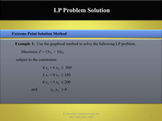
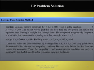
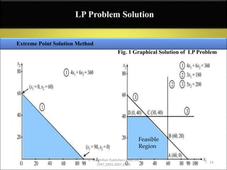
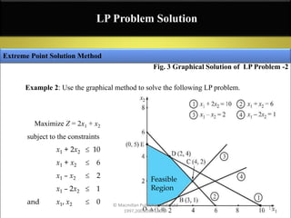
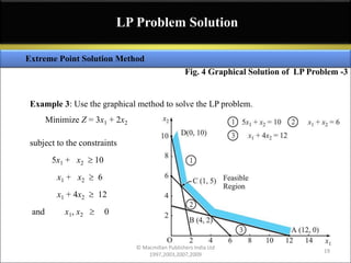
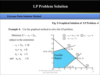
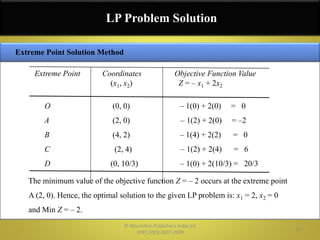
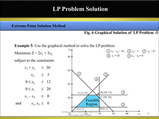
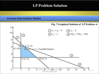
Lecture5-7_12946_Linear Programming The Graphical Method.pptx

Linear Programming: The
Graphical Method
1
© Macmillan Publishers India Ltd
1997,2003,2007,2009

“People realize that[technology]certainly is a tool.
This tool can be used to enhance operations, Improve
efficiencies and really add value to academic
research and teaching exercises.”
Peter Murray
2
1997,2003,2007,2009

LP Problem Solution
An optimal, as well as feasible solution to an LP problem is obtained by
choosing from several values of decision variables x1, x2, . . ., xn, the one set of
values that satisfies the given set of constraints simultaneously and also provides
the optimal (maximum or minimum) value of the given objective function.
LP problems with two variables, the entire set of feasible solutions can be
displayed graphically by plotting linear constraints on a graph paper to best
(optimal) solution. The technique used to identify the optimal solution is called
the graphical solution approach.
This solution approach provides valuable understanding of how to solve LP
problems involving more than two variables algebraically.
3
1997,2003,2007,2009

Graphical solution methods (or approaches) are:
Iso-profit (cost) function line method used to find the optimal solution to an LP problem.
Extreme point solution method
LP Problem Solution
4
1997,2003,2007,2009

Feasible solution: The set of values of decision variables xj (j = 1, 2, . . ., n) which satisfy all the
constraints and non-negativity conditions of an LP problem simultaneously is said to
constitute the feasible solution to that LP problem.
Infeasible solution: The set of values of decision variables xj ( j = 1, 2, . . ., n) which do not
satisfy all the constraints and non-negativity conditions of an LP problem simultaneously is
said to constitute the infeasible solution to that LP problem.
Solution: The set of values of decision variables xj (j = 1, 2, . . ., n) which satisfy the constraints
of an LP problem is said to constitute solution to that LP problem.
Important Definitions
LP Problem Solution
5
1997,2003,2007,2009

Basic feasible solution: A feasible solution to an LP problem which is also the basic solution is
called the basic feasible solution. That is, all basic variables assume non-negative values. Basic
feasible solutions are of two types:
Basic solution: For a set of m simultaneous equations in n variables (n > m), a solution obtained
by setting (n – m) variables equal to zero and solving for remaining m equations in m variables is
called a basic solution.
The (n – m) variables whose value did not appear in this solution are called non-basic
variables and the remaining m variables are called basic variables.
Degenerate: A basic feasible solution is called degenerate if value of at least one basic
variable is zero.
Non-degenerate: A basic feasible solution is called non-degenerate if values of all m basic
variables are non-zero and positive
LP Problem Solution
6
1997,2003,2007,2009

Optimum basic feasible solution: A basic feasible solution which optimizes (maximizes or
minimizes) the objective function value of the given LP problem is called an optimum
basic feasible solution.
Unbounded solution : A solution which can increase or decrease the value of objective
function of the LP problem indefinitely is called an unbounded solution.
LP Problem Solution
7
1997,2003,2007,2009

While obtaining the optimal solution to the LP problem by the graphical method, the statement
of the following theorems is used.
LP Problem Solution
Standard Results
 The collection of all feasible solutions to an LP problem constitutes a convex set whose
extreme points correspond to the basic feasible solutions.
 If the optimal solution occurs at more than one extreme point, the value of the objective
function will be the same for all convex combinations of these extreme points.
 There are a finite number of basic feasible solutions within the feasible solution space.
 If the convex set of the feasible solutions of the system of simultaneous equations: Ax
= b, x  0 , is a convex polyhedron, then at least one of the extreme points gives an
optimal solution.
8
1997,2003,2007,2009

LP Problem Solution
Step 1:Develop LP model:
Extreme Point Solution Method
Coordinates of all corner (or extreme) points of the feasible region (space or area)
are determined and then values of the objective function at these points are
computed and compared because an optimal solution to any LP problem always lie
at one of the corner (extreme) points of the feasible solution space.
Step 2:Plot constraints on graph paper and decide the feasible region
State the given problem in the mathematical LP model.
Draw these straight lines on the graph paper and decide each time the area of feasible solutions
according to the inequality sign of the constraint. Shade the common portion of the graph
that satisfies all the constraints simultaneously drawn so far.
Replace the inequality sign in each constraint by an equality sign.
9
1997,2003,2007,2009

LP Problem Solution
The final shaded area is called the feasible region (or solution space) of the given LP problem.
Any point inside this region is called feasible solution and provides values of x1 and x2 that
satisfy all constraints.
Step 3:Examine extreme points of the feasible solution space to find an optimal solution
Identify extreme point that gives optimal (max. or min.) value of the objective function.
Compute and compare the value of the objective function at each extreme point.
Determine the coordinates of each extreme point of the feasible solution space.
10
1997,2003,2007,2009

LP Problem Solution
Example 1: Use the graphical method to solve the following LP problem.
Maximize Z = 15x1 + 10x2
subject to the constraints
4 x1 + 6 x2  360
3 x1 + 0 x2  180
0 x1 + 5 x2  200
and x1, x2  0
11
1997,2003,2007,2009

LP Problem Solution
Soution: Consider the first constraint 4 x1 + 6 x2  360. Treat it as the equation, 4
x1 + 6 x2 = 360. The easiest way to plot this line is to find any two points that satisfy the
equation, then drawing a straight line through them. The two points are generally the points
at which the line intersects the x1 and x2 axes. For example, when x1 = 0
we get 6 x2 = 360 or x2 = 60. Similarly when x2 = 0, 4 x1 = 360, x1 = 90
These two points are then connected by a straight line 4 x1 + 6 x2  360. Any point above
the constraint line violates the inequality condition. But any point below the line does not
violate the constraint. Thus, the inequality and non-negativity condition can only be
satisfied by the shaded area (feasible region) as shown in the figure.
12
1997,2003,2007,2009

LP Problem Solution
Similarly, the constraints 3 x1  180 and 5 x2  200 are also plotted on the graph and are indicated
by the shaded area in the figure.
Since all constraints have been graphed, the area which is bounded by all the constraints lines
including all the boundary points is called the feasible region (or solution space). The
feasible region is shown by the shaded area OABCD in the figure.
13
1997,2003,2007,2009

LP Problem Solution
Fig. 1 Graphical Solution of LP Problem
Feasible
Region
14
1997,2003,2007,2009

LP Problem Solution
i) Since the optimal value of the objective function occurs at one of the extreme
points of the feasible region, it is necessary to determine their coordinates. The
coordinates of extreme points of the feasible region are: O = (0, 0), A = (60,
0), B = (60, 20), C = (30, 40), D = (0, 40).
ii) Evaluate objective function value at each extreme point of the feasible region
Extreme Point Coordinates Objective Function Value
(x1, x2) Z = 15x1 + 10x2
O (0, 0) 15(0) + 10(0) = 0
A (60, 0) 15(60) + 10(0) = 900
B (60, 20) 15(60) + 10(20) = 1,100
C (30, 40) 5(30) + 10(40) = 850
D (0, 40) 15(0) + 10(40) = 400
15
1997,2003,2007,2009

LP Problem Solution
iii) Since maximum value of Z = 1,100 is achieved at the point extreme B (60, 20).
Hence the optimal solution to the given LP problem is: x1 = 60, x2 = 20 and
Max Z = 1,100
16
1997,2003,2007,2009

LP Problem Solution
Example 2: Use the graphical method to solve the following LP problem.
Maximize Z = 2x1 + x2
x1 + 2x2  10
x1 + x2  6
x1 – x2  2
x1 – 2x2  1
and x1, x2  0
Feasible
Region
Fig. 3 Graphical Solution of LP Problem -2
17
1997,2003,2007,2009

(x1, x2) Z = 2x1 + x2
O (0, 0) 2(0) + 1(0) = 0
A (1, 0) 2(1) + 1(0) = 2
B (3, 1) 2(3) + 1(1) = 7
C (4, 2) 2(4) + 1(2) = 10
D (2, 4) 2(2) + 1(4) = 8
E (0, 5) 2(0) + 1(5) = 5
The maximum value of the objective function Z = 10 occurs at the extreme point
(4,2). Hence, the optimal solution to the given LP problem is: x1 = 4, x2 = 2 and
Max Z = 10.
LP Problem Solution
18
1997,2003,2007,2009

LP Problem Solution
Example 3: Use the graphical method to solve the LP problem.
Minimize Z = 3x1 + 2x2
5x1 + x2  10
x1 + x2 6
x1 + 4x2 12
and x1, x2  0
19
1997,2003,2007,2009

LP Problem Solution
(x1, x2) Z = 3x1 + 2x2
A (12, 0) 3(12) + 2(0) = 36
B (4, 2) 3(4) + 2(2) = 16
C (1, 5) 3(1) + 2(5) = 13
D (0, 10) 3(0) + 2(10) = 20
The minimum value of the objective function Z = 13 occurs at the extreme point
C (1, 5). Hence, the optimal solution to the given LP problem is:
x1 = 1, x2 = 5, and Min Z = 13. 20
1997,2003,2007,2009

LP Problem Solution
Minimize Z = – x1 + 2x2
– x1 + 3x2  10
x1 + x2  6
x1 – x2  2
and x1, x2  0.
Feasible
Region
21
1997,2003,2007,2009

LP Problem Solution
(x1, x2) Z = – x1 + 2x2
O (0, 0) – 1(0) + 2(0) = 0
A (2, 0) – 1(2) + 2(0) = –2
B (4, 2) – 1(4) + 2(2) = 0
C (2, 4) – 1(2) + 2(4) = 6
D (0, 10/3) – 1(0) + 2(10/3) = 20/3
The minimum value of the objective function Z = – 2 occurs at the extreme point
A (2, 0). Hence, the optimal solution to the given LP problem is: x1 = 2, x2 = 0
and Min Z = – 2.
22
1997,2003,2007,2009

LP Problem Solution
Maximize Z = 2x1 + 3x2
x1 + x2  30
x2  3
0  x2 12
0 x1 20
x1 – x2  0
and x1, x2  0
Feasible
Region
23
1997,2003,2007,2009

LP Problem Solution
(x1, x2) Z = 2x1 + 3x2
A (3, 3) 2(3) + 3(3) = 15
B (20, 3) 2(20) + 3(3) = 49
C (20, 10) 2(20) + 3(10) = 70
D (18, 12) 2(18) + 3(12) = 72
E (12, 12) 2(12) + 3(12) = 60
The maximum value of the objective function Z = 72 occurs at the extreme point
D (18,12). Hence, the optimal solution to the given LP problem is: x1 = 18, x2 = 12
and Max Z = 72 24
1997,2003,2007,2009

LP Problem Solution
Example 6: A firm makes two products X and Y, and has a total production
capacity of 9 tones per day, X and Y requiring the same production capacity. The
firm has a permanent contract to supply at least 2 tones of X and at least 3 tones
of Y per day to another company. Each tone of X requires 20 machine hours of
production time and each tone of Y requires 50 machine hours of production time.
The daily maximum possible number of machine hours is 360. All the firm’s
output can be sold, and the profit made is Rs. 80 per tone of X and Rs. 120 per
tone of Y. It is required to determine the production schedule for maximum profit
and to calculate this profit.
25
1997,2003,2007,2009

LP Problem Solution
(x1, x2) Z = 80x1 + 120x2
A (2, 3) 80(2) + 120(3) = 520
B (6, 3) 80(6) + 120(3) = 840
C (3, 6) 80(3) + 120(6) = 960
D (2, 6.4) 80(2) + 120(6.4) = 928
The maximum value of the objective function Z = 960 occurs at the extreme
point C (3, 6). Hence the company should produce, x1 = 3 tones of product X
and x2 = 6 tones of product Y in order to yield a maximum profit of Rs. 960.
26
1997,2003,2007,2009

LP Problem Solution
27
1997,2003,2007,2009

LP Problem Solution
Example 7: A manufacturer produces two different models: X and Y, of the same
product. Model X makes a contribution of Rs 50 per unit and model Y, Rs 30 per
unit towards total profit. Raw materials r1 and r2 are required for production. At
least 18 kg of r1 and 12 kg of r2 must be used daily. Also at most 34 hours of
labour are to be utilized.
A quantity of 2 kg of r1 is needed for model X and 1 kg of r1 for model Y. For
each of X and Y, 1 kg of r2 is required. It takes 3 hours to manufacture model X
and 2 hours to manufacture model Y. How many units of each model should be
produced to maximize the profit?
28
1997,2003,2007,2009

LP Problem Solution
Fig. 8 Graphical Solution of LP Problem - 7
29
1997,2003,2007,2009

LP Problem Solution
(x1, x2) Z = 50x1 + 30x2
A (6, 6) 50(6) + 30(6) = 480
B (2, 14) 50(2) + 30(14) = 520
C (10, 2) 50(10) + 30(2) = 560
Since the maximum value of Z = 560 occurs at the point C (10, 2), the
manufacturer should produce x1 = 10 units of model X and x2 = 2 units of Y to
yield a maximum profit of Rs. 560.
30
1997,2003,2007,2009

Lecture5-7_12946_Linear Programming The Graphical Method.pptx

More Related Content

Similar to Lecture5-7_12946_Linear Programming The Graphical Method.pptx

More from hlKh4

Recently uploaded

Lecture5-7_12946_Linear Programming The Graphical Method.pptx