Download as PDF, PPTX

![eHS uses the modified nodal analysis approach
– It solves a admittance matrix to find the voltage at each node and the current from each sources.
– The admittance matrix does not need to be re-computed for each switch status
– Simulated model topology and parameters can be modified without recompiling the bitstream
The maximum size of the circuit is determined by the number of inputs,
switches and reactive components
Currently, the maximum number of components is :
– 16 inputs (voltage/current sources)
– 16 outputs (voltage/current measurements)
– 24 switches (IGBTs, breakers, etc)
– 60 non-switching devices (ie. L and C) – unlimited resistors
eHS Nodal Solver
eHS core
Y[0:15]
24x switches control
16x Inputs
U[0:15]
S[0:23]
16 Measurements](https://image.slidesharecdn.com/opalrtrealtimesimulationusingrtlabcompel2013-140819152645-phpapp02/85/OPAL-RT-Real-time-simulation-using-RT-LAB-15-320.jpg)
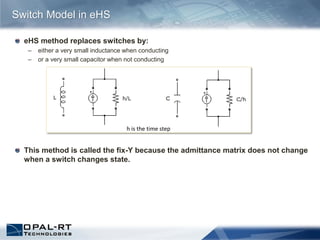

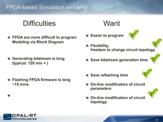
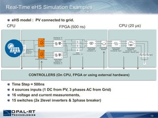
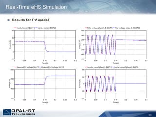
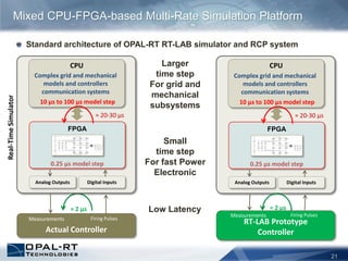

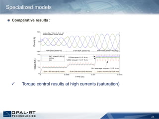
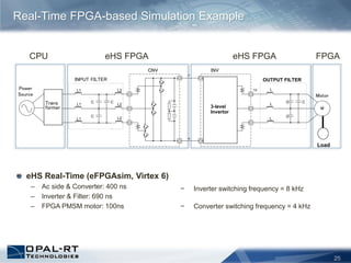
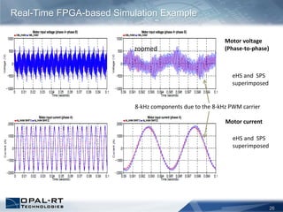
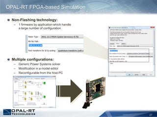


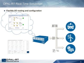
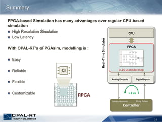


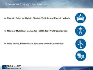
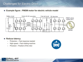
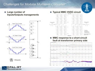
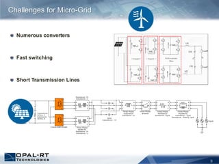
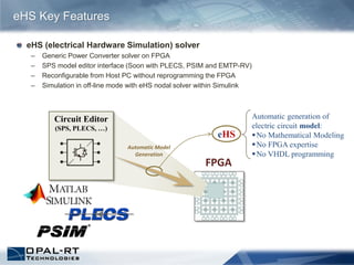
This document discusses using real-time simulation with FPGA-based hardware to model renewable energy systems. It describes challenges in modeling electric drives, modular multilevel converters, microgrids, and other renewable energy technologies. The document introduces OPAL-RT's eHS solution for modeling power electronics circuits on FPGAs for real-time simulation. eHS allows generating circuit models automatically without programming FPGAs directly. Examples are presented showing an eHS model of a PV system connected to the grid running in real-time on an FPGA. Real-time FPGA simulation provides benefits over CPU simulation like higher resolution, lower latency, and specialized models.