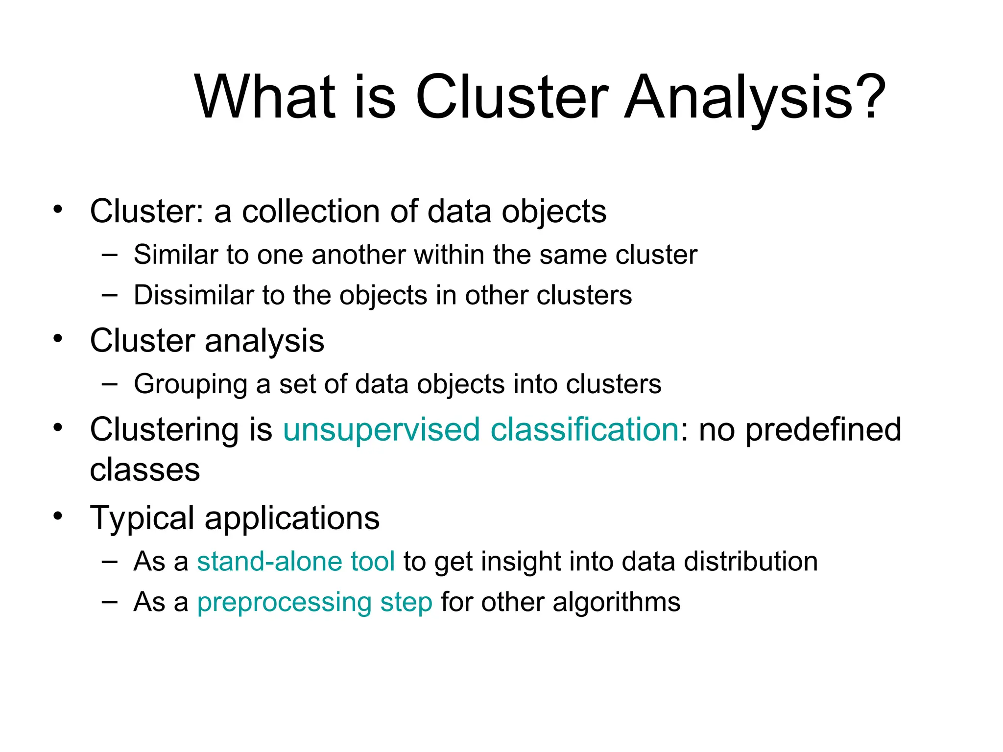
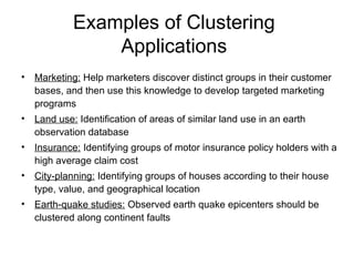
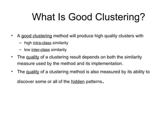
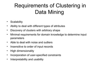
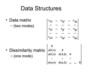
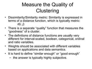
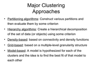
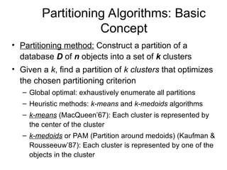
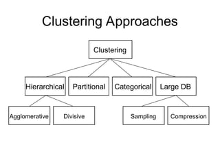
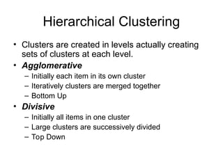
What is Cluster Analysis?
• Cluster: a collection of data objects
– Similar to one another within the same cluster
– Dissimilar to the objects in other clusters
• Cluster analysis
– Grouping a set of data objects into clusters
• Clustering is unsupervised classification: no predefined
classes
• Typical applications
– As a stand-alone tool to get insight into data distribution
– As a preprocessing step for other algorithms
Examples of Clustering
Applications
• Marketing: Help marketers discover distinct groups in their customer
bases, and then use this knowledge to develop targeted marketing
programs
• Land use: Identification of areas of similar land use in an earth
observation database
• Insurance: Identifying groups of motor insurance policy holders with a
high average claim cost
• City-planning: Identifying groups of houses according to their house
type, value, and geographical location
• Earth-quake studies: Observed earth quake epicenters should be
clustered along continent faults
What Is Good Clustering?
• A good clustering method will produce high quality clusters with
– high intra-class similarity
– low inter-class similarity
• The quality of a clustering result depends on both the similarity
measure used by the method and its implementation.
• The quality of a clustering method is also measured by its ability to
discover some or all of the hidden patterns.
Requirements of Clustering in
Data Mining
• Scalability
• Ability to deal with different types of attributes
• Discovery of clusters with arbitrary shape
• Minimal requirements for domain knowledge to determine input
parameters
• Able to deal with noise and outliers
• Insensitive to order of input records
• High dimensionality
• Incorporation of user-specified constraints
• Interpretability and usability
Data Structures
• Data matrix
– (two modes)
• Dissimilarity matrix
– (one mode)


















np
x
...
nf
x
...
n1
x
...
...
...
...
...
ip
x
...
if
x
...
i1
x
...
...
...
...
...
1p
x
...
1f
x
...
11
x
















0
...
)
2
,
(
)
1
,
(
:
:
:
)
2
,
3
(
)
...
n
d
n
d
0
d
d(3,1
0
d(2,1)
0
Measure the Quality of
Clustering
• Dissimilarity/Similarity metric: Similarity is expressed in
terms of a distance function, which is typically metric:
d(i, j)
• There is a separate “quality” function that measures the
“goodness” of a cluster.
• The definitions of distance functions are usually very
different for interval-scaled, boolean, categorical, ordinal
and ratio variables.
• Weights should be associated with different variables
based on applications and data semantics.
• It is hard to define “similar enough” or “good enough”
– the answer is typically highly subjective.
Major Clustering
Approaches
• Partitioning algorithms: Construct various partitions and
then evaluate them by some criterion
• Hierarchy algorithms: Create a hierarchical decomposition
of the set of data (or objects) using some criterion
• Density-based: based on connectivity and density functions
• Grid-based: based on a multiple-level granularity structure
• Model-based: A model is hypothesized for each of the
clusters and the idea is to find the best fit of that model to
each other
Partitioning Algorithms: Basic
Concept
• Partitioning method: Construct a partition of a
database D of n objects into a set of k clusters
• Given a k, find a partition of k clusters that optimizes
the chosen partitioning criterion
– Global optimal: exhaustively enumerate all partitions
– Heuristic methods: k-means and k-medoids algorithms
– k-means (MacQueen’67): Each cluster is represented by
the center of the cluster
– k-medoids or PAM (Partition around medoids) (Kaufman &
Rousseeuw’87): Each cluster is represented by one of the
objects in the cluster
The K-Means Clustering Method
• Given k, the k-means algorithm is implemented
in four steps:
– Partition objects into k nonempty subsets
– Compute seed points as the centroids of the clusters
of the current partition (the centroid is the center, i.e.,
mean point, of the cluster)
– Assign each object to the cluster with the nearest
seed point
– Go back to Step 2, stop when no more new
assignment
The K-Means Clustering Method
• Example
0
1
2
3
4
5
6
7
8
9
10
0 1 2 3 4 5 6 7 8 9 10
0
1
2
3
4
5
6
7
8
9
10
0 1 2 3 4 5 6 7 8 9 10
0
1
2
3
4
5
6
7
8
9
10
0 1 2 3 4 5 6 7 8 9 10
0
1
2
3
4
5
6
7
8
9
10
0 1 2 3 4 5 6 7 8 9 10
0
1
2
3
4
5
6
7
8
9
10
0 1 2 3 4 5 6 7 8 9 10
K=2
Arbitrarily choose K
object as initial
cluster center
Assign
each
objects
to most
similar
center
Update
the
cluster
means
Update
the
cluster
means
reassign
reassign
Comments on the K-Means
Method
• Strength: Relatively efficient: O(tkn), where n is #
objects, k is # clusters, and t is # iterations. Normally, k,
t << n.
• Comparing: PAM: O(k(n-k)2
), CLARA: O(ks2
+ k(n-k))
• Weakness
– Applicable only when mean is defined, then what about
categorical data?
– Need to specify k, the number of clusters, in advance
– Unable to handle noisy data and outliers
– Not suitable to discover clusters with non-convex shapes
Variations of the K-Means Method
• A few variants of the k-means which differ in
– Selection of the initial k means
– Dissimilarity calculations
– Strategies to calculate cluster means
• Handling categorical data: k-modes (Huang’98)
– Replacing means of clusters with modes
– Using new dissimilarity measures to deal with categorical objects
– Using a frequency-based method to update modes of clusters
– A mixture of categorical and numerical data: k-prototype method
What is the problem of k-Means
Method?
• The k-means algorithm is sensitive to outliers !
– Since an object with an extremely large value may substantially distort the
distribution of the data.
• K-Medoids: Instead of taking the mean value of the object in a cluster as a
reference point, medoids can be used, which is the most centrally located
object in a cluster.
0
1
2
3
4
5
6
7
8
9
10
0 1 2 3 4 5 6 7 8 9 10
0
1
2
3
4
5
6
7
8
9
10
0 1 2 3 4 5 6 7 8 9 10
The K-Medoids Clustering Method
• Find representative objects, called medoids, in clusters
• PAM (Partitioning Around Medoids, 1987)
– starts from an initial set of medoids and iteratively replaces one of the
medoids by one of the non-medoids if it improves the total distance of
the resulting clustering
– PAM works effectively for small data sets, but does not scale well for
large data sets
• CLARA (Kaufmann & Rousseeuw, 1990)
• CLARANS (Ng & Han, 1994): Randomized sampling
• Focusing + spatial data structure (Ester et al., 1995)
Typical k-medoids algorithm (PAM)
0
1
2
3
4
5
6
7
8
9
10
0 1 2 3 4 5 6 7 8 9 10
Total Cost = 20
0
1
2
3
4
5
6
7
8
9
10
0 1 2 3 4 5 6 7 8 9 10
K=2
Arbitrar
y choose
k object
as initial
medoids
0
1
2
3
4
5
6
7
8
9
10
0 1 2 3 4 5 6 7 8 9 10
Assign
each
remaini
ng
object to
nearest
medoids
Randomly select a
nonmedoid
object,Oramdom
Compute
total cost
of
swapping
0
1
2
3
4
5
6
7
8
9
10
0 1 2 3 4 5 6 7 8 9 10
Total Cost = 26
Swapping O
and Oramdom
If quality is
improved.
Do loop
Until no
change
0
1
2
3
4
5
6
7
8
9
10
0 1 2 3 4 5 6 7 8 9 10
PAM (Partitioning Around Medoids) (1987)
• PAM (Kaufman and Rousseeuw, 1987), built in Splus
• Use real object to represent the cluster
– Select k representative objects arbitrarily
– For each pair of non-selected object h and selected object i,
calculate the total swapping cost TCih
– For each pair of i and h,
• If TCih < 0, i is replaced by h
• Then assign each non-selected object to the most similar
representative object
– repeat steps 2-3 until there is no change
PAM Clustering: Total swapping cost
TCih=jCjih
0
1
2
3
4
5
6
7
8
9
10
0 1 2 3 4 5 6 7 8 9 10
j
i
h
t
Cjih = 0
0
1
2
3
4
5
6
7
8
9
10
0 1 2 3 4 5 6 7 8 9 10
t
i h
j
Cjih = d(j, h) - d(j, i)
0
1
2
3
4
5
6
7
8
9
10
0 1 2 3 4 5 6 7 8 9 10
h
i
t
j
Cjih = d(j, t) - d(j, i)
0
1
2
3
4
5
6
7
8
9
10
0 1 2 3 4 5 6 7 8 9 10
t
i
h j
Cjih = d(j, h) - d(j, t)
What is the problem with PAM?
• Pam is more robust than k-means in the presence of noise
and outliers because a medoid is less influenced by outliers
or other extreme values than a mean
• Pam works efficiently for small data sets but does not scale
well for large data sets.
– O(k(n-k)2
) for each iteration
where n is # of data,k is # of clusters
Sampling based method,
CLARA(Clustering LARge Applications)
CLARA (Clustering Large Applications) (1990)
• CLARA (Kaufmann and Rousseeuw in 1990)
– Built in statistical analysis packages, such as S+
• It draws multiple samples of the data set, applies PAM on each
sample, and gives the best clustering as the output
• Strength: deals with larger data sets than PAM
• Weakness:
– Efficiency depends on the sample size
– A good clustering based on samples will not necessarily represent a
good clustering of the whole data set if the sample is biased
K-Means Example
• Given: {2,4,10,12,3,20,30,11,25}, k=2
• Randomly assign means: m1=3,m2=4
• Solve for the rest ….
• Similarly try for k-medoids
Clustering Approaches
Clustering
Hierarchical Partitional Categorical Large DB
Agglomerative Divisive Sampling Compression
Cluster Summary Parameters
Distance Between Clusters
• Single Link: smallest distance between points
• Complete Link: largest distance between points
• Average Link: average distance between points
• Centroid: distance between centroids
Hierarchical Clustering
• Use distance matrix as clustering criteria. This method does not
require the number of clusters k as an input, but needs a
termination condition
Step 0 Step 1 Step 2 Step 3 Step 4
b
d
c
e
a
a b
d e
c d e
a b c d e
Step 4 Step 3 Step 2 Step 1 Step 0
agglomerative
(AGNES)
divisive
(DIANA)
Hierarchical Clustering
• Clusters are created in levels actually creating
sets of clusters at each level.
• Agglomerative
– Initially each item in its own cluster
– Iteratively clusters are merged together
– Bottom Up
• Divisive
– Initially all items in one cluster
– Large clusters are successively divided
– Top Down
Hierarchical Algorithms
• Single Link
• MST Single Link
• Complete Link
• Average Link
Dendrogram
• Dendrogram: a tree data
structure which illustrates
hierarchical clustering
techniques.
• Each level shows clusters for
that level.
– Leaf – individual clusters
– Root – one cluster
• A cluster at level i is the union
of its children clusters at level
i+1.
Levels of Clustering
Agglomerative Example
A B C D E
A 0 1 2 2 3
B 1 0 2 4 3
C 2 2 0 1 5
D 2 4 1 0 3
E 3 3 5 3 0
B
A
E C
D
4
Threshold of
2 3 5
1
A B C D E
MST Example
A B C D E
A 0 1 2 2 3
B 1 0 2 4 3
C 2 2 0 1 5
D 2 4 1 0 3
E 3 3 5 3 0
B
A
E C
D
Agglomerative Algorithm
Single Link
• View all items with links (distances) between them.
• Finds maximal connected components in this graph.
• Two clusters are merged if there is at least one edge
which connects them.
• Uses threshold distances at each level.
• Could be agglomerative or divisive.
MST Single Link Algorithm
Single Link Clustering
AGNES (Agglomerative
Nesting)
• Introduced in Kaufmann and Rousseeuw (1990)
• Implemented in statistical analysis packages, e.g., Splus
• Use the Single-Link method and the dissimilarity matrix.
• Merge nodes that have the least dissimilarity
• Go on in a non-descending fashion
• Eventually all nodes belong to the same cluster
0
1
2
3
4
5
6
7
8
9
10
0 1 2 3 4 5 6 7 8 9 10
0
1
2
3
4
5
6
7
8
9
10
0 1 2 3 4 5 6 7 8 9 10
0
1
2
3
4
5
6
7
8
9
10
0 1 2 3 4 5 6 7 8 9 10
DIANA (Divisive Analysis)
• Introduced in Kaufmann and Rousseeuw (1990)
• Implemented in statistical analysis packages, e.g., Splus
• Inverse order of AGNES
• Eventually each node forms a cluster on its own
0
1
2
3
4
5
6
7
8
9
10
0 1 2 3 4 5 6 7 8 9 10
0
1
2
3
4
5
6
7
8
9
10
0 1 2 3 4 5 6 7 8 9 10
0
1
2
3
4
5
6
7
8
9
10
0 1 2 3 4 5 6 7 8 9 10
Readings
• CHAMELEON: A Hierarchical Clustering Algorithm Using Dynamic
Modeling. George Karypis, Eui-Hong Han, Vipin Kumar, IEEE Computer
32(8): 68-75, 1999 (http://glaros.dtc.umn.edu/gkhome/node/152)
• A Density-Based Algorithm for Discovering Clusters in Large Spatial
Databases with Noise. Martin Ester, Hans-Peter Kriegel, Jörg Sander,
Xiaowei Xu. Proceedings of 2nd International Conference on Knowledge
Discovery and Data Mining (KDD-96)
• BIRCH: A New Data Clustering Algorithm and Its Applications. Data Mining
and Knowledge Discovery Volume 1 , Issue 2 (1997)

2002_Spring_CS525_Lggggggfdtfffdfgecture_2.ppt

  • 1.
    What is ClusterAnalysis? • Cluster: a collection of data objects – Similar to one another within the same cluster – Dissimilar to the objects in other clusters • Cluster analysis – Grouping a set of data objects into clusters • Clustering is unsupervised classification: no predefined classes • Typical applications – As a stand-alone tool to get insight into data distribution – As a preprocessing step for other algorithms
  • 2.
    Examples of Clustering Applications •Marketing: Help marketers discover distinct groups in their customer bases, and then use this knowledge to develop targeted marketing programs • Land use: Identification of areas of similar land use in an earth observation database • Insurance: Identifying groups of motor insurance policy holders with a high average claim cost • City-planning: Identifying groups of houses according to their house type, value, and geographical location • Earth-quake studies: Observed earth quake epicenters should be clustered along continent faults
  • 3.
    What Is GoodClustering? • A good clustering method will produce high quality clusters with – high intra-class similarity – low inter-class similarity • The quality of a clustering result depends on both the similarity measure used by the method and its implementation. • The quality of a clustering method is also measured by its ability to discover some or all of the hidden patterns.
  • 4.
    Requirements of Clusteringin Data Mining • Scalability • Ability to deal with different types of attributes • Discovery of clusters with arbitrary shape • Minimal requirements for domain knowledge to determine input parameters • Able to deal with noise and outliers • Insensitive to order of input records • High dimensionality • Incorporation of user-specified constraints • Interpretability and usability
  • 5.
    Data Structures • Datamatrix – (two modes) • Dissimilarity matrix – (one mode)                   np x ... nf x ... n1 x ... ... ... ... ... ip x ... if x ... i1 x ... ... ... ... ... 1p x ... 1f x ... 11 x                 0 ... ) 2 , ( ) 1 , ( : : : ) 2 , 3 ( ) ... n d n d 0 d d(3,1 0 d(2,1) 0
  • 6.
    Measure the Qualityof Clustering • Dissimilarity/Similarity metric: Similarity is expressed in terms of a distance function, which is typically metric: d(i, j) • There is a separate “quality” function that measures the “goodness” of a cluster. • The definitions of distance functions are usually very different for interval-scaled, boolean, categorical, ordinal and ratio variables. • Weights should be associated with different variables based on applications and data semantics. • It is hard to define “similar enough” or “good enough” – the answer is typically highly subjective.
  • 7.
    Major Clustering Approaches • Partitioningalgorithms: Construct various partitions and then evaluate them by some criterion • Hierarchy algorithms: Create a hierarchical decomposition of the set of data (or objects) using some criterion • Density-based: based on connectivity and density functions • Grid-based: based on a multiple-level granularity structure • Model-based: A model is hypothesized for each of the clusters and the idea is to find the best fit of that model to each other
  • 8.
    Partitioning Algorithms: Basic Concept •Partitioning method: Construct a partition of a database D of n objects into a set of k clusters • Given a k, find a partition of k clusters that optimizes the chosen partitioning criterion – Global optimal: exhaustively enumerate all partitions – Heuristic methods: k-means and k-medoids algorithms – k-means (MacQueen’67): Each cluster is represented by the center of the cluster – k-medoids or PAM (Partition around medoids) (Kaufman & Rousseeuw’87): Each cluster is represented by one of the objects in the cluster
  • 9.
    The K-Means ClusteringMethod • Given k, the k-means algorithm is implemented in four steps: – Partition objects into k nonempty subsets – Compute seed points as the centroids of the clusters of the current partition (the centroid is the center, i.e., mean point, of the cluster) – Assign each object to the cluster with the nearest seed point – Go back to Step 2, stop when no more new assignment
  • 10.
    The K-Means ClusteringMethod • Example 0 1 2 3 4 5 6 7 8 9 10 0 1 2 3 4 5 6 7 8 9 10 0 1 2 3 4 5 6 7 8 9 10 0 1 2 3 4 5 6 7 8 9 10 0 1 2 3 4 5 6 7 8 9 10 0 1 2 3 4 5 6 7 8 9 10 0 1 2 3 4 5 6 7 8 9 10 0 1 2 3 4 5 6 7 8 9 10 0 1 2 3 4 5 6 7 8 9 10 0 1 2 3 4 5 6 7 8 9 10 K=2 Arbitrarily choose K object as initial cluster center Assign each objects to most similar center Update the cluster means Update the cluster means reassign reassign
  • 11.
    Comments on theK-Means Method • Strength: Relatively efficient: O(tkn), where n is # objects, k is # clusters, and t is # iterations. Normally, k, t << n. • Comparing: PAM: O(k(n-k)2 ), CLARA: O(ks2 + k(n-k)) • Weakness – Applicable only when mean is defined, then what about categorical data? – Need to specify k, the number of clusters, in advance – Unable to handle noisy data and outliers – Not suitable to discover clusters with non-convex shapes
  • 12.
    Variations of theK-Means Method • A few variants of the k-means which differ in – Selection of the initial k means – Dissimilarity calculations – Strategies to calculate cluster means • Handling categorical data: k-modes (Huang’98) – Replacing means of clusters with modes – Using new dissimilarity measures to deal with categorical objects – Using a frequency-based method to update modes of clusters – A mixture of categorical and numerical data: k-prototype method
  • 13.
    What is theproblem of k-Means Method? • The k-means algorithm is sensitive to outliers ! – Since an object with an extremely large value may substantially distort the distribution of the data. • K-Medoids: Instead of taking the mean value of the object in a cluster as a reference point, medoids can be used, which is the most centrally located object in a cluster. 0 1 2 3 4 5 6 7 8 9 10 0 1 2 3 4 5 6 7 8 9 10 0 1 2 3 4 5 6 7 8 9 10 0 1 2 3 4 5 6 7 8 9 10
  • 14.
    The K-Medoids ClusteringMethod • Find representative objects, called medoids, in clusters • PAM (Partitioning Around Medoids, 1987) – starts from an initial set of medoids and iteratively replaces one of the medoids by one of the non-medoids if it improves the total distance of the resulting clustering – PAM works effectively for small data sets, but does not scale well for large data sets • CLARA (Kaufmann & Rousseeuw, 1990) • CLARANS (Ng & Han, 1994): Randomized sampling • Focusing + spatial data structure (Ester et al., 1995)
  • 15.
    Typical k-medoids algorithm(PAM) 0 1 2 3 4 5 6 7 8 9 10 0 1 2 3 4 5 6 7 8 9 10 Total Cost = 20 0 1 2 3 4 5 6 7 8 9 10 0 1 2 3 4 5 6 7 8 9 10 K=2 Arbitrar y choose k object as initial medoids 0 1 2 3 4 5 6 7 8 9 10 0 1 2 3 4 5 6 7 8 9 10 Assign each remaini ng object to nearest medoids Randomly select a nonmedoid object,Oramdom Compute total cost of swapping 0 1 2 3 4 5 6 7 8 9 10 0 1 2 3 4 5 6 7 8 9 10 Total Cost = 26 Swapping O and Oramdom If quality is improved. Do loop Until no change 0 1 2 3 4 5 6 7 8 9 10 0 1 2 3 4 5 6 7 8 9 10
  • 16.
    PAM (Partitioning AroundMedoids) (1987) • PAM (Kaufman and Rousseeuw, 1987), built in Splus • Use real object to represent the cluster – Select k representative objects arbitrarily – For each pair of non-selected object h and selected object i, calculate the total swapping cost TCih – For each pair of i and h, • If TCih < 0, i is replaced by h • Then assign each non-selected object to the most similar representative object – repeat steps 2-3 until there is no change
  • 17.
    PAM Clustering: Totalswapping cost TCih=jCjih 0 1 2 3 4 5 6 7 8 9 10 0 1 2 3 4 5 6 7 8 9 10 j i h t Cjih = 0 0 1 2 3 4 5 6 7 8 9 10 0 1 2 3 4 5 6 7 8 9 10 t i h j Cjih = d(j, h) - d(j, i) 0 1 2 3 4 5 6 7 8 9 10 0 1 2 3 4 5 6 7 8 9 10 h i t j Cjih = d(j, t) - d(j, i) 0 1 2 3 4 5 6 7 8 9 10 0 1 2 3 4 5 6 7 8 9 10 t i h j Cjih = d(j, h) - d(j, t)
  • 18.
    What is theproblem with PAM? • Pam is more robust than k-means in the presence of noise and outliers because a medoid is less influenced by outliers or other extreme values than a mean • Pam works efficiently for small data sets but does not scale well for large data sets. – O(k(n-k)2 ) for each iteration where n is # of data,k is # of clusters Sampling based method, CLARA(Clustering LARge Applications)
  • 19.
    CLARA (Clustering LargeApplications) (1990) • CLARA (Kaufmann and Rousseeuw in 1990) – Built in statistical analysis packages, such as S+ • It draws multiple samples of the data set, applies PAM on each sample, and gives the best clustering as the output • Strength: deals with larger data sets than PAM • Weakness: – Efficiency depends on the sample size – A good clustering based on samples will not necessarily represent a good clustering of the whole data set if the sample is biased
  • 20.
    K-Means Example • Given:{2,4,10,12,3,20,30,11,25}, k=2 • Randomly assign means: m1=3,m2=4 • Solve for the rest …. • Similarly try for k-medoids
  • 21.
    Clustering Approaches Clustering Hierarchical PartitionalCategorical Large DB Agglomerative Divisive Sampling Compression
  • 22.
  • 23.
    Distance Between Clusters •Single Link: smallest distance between points • Complete Link: largest distance between points • Average Link: average distance between points • Centroid: distance between centroids
  • 24.
    Hierarchical Clustering • Usedistance matrix as clustering criteria. This method does not require the number of clusters k as an input, but needs a termination condition Step 0 Step 1 Step 2 Step 3 Step 4 b d c e a a b d e c d e a b c d e Step 4 Step 3 Step 2 Step 1 Step 0 agglomerative (AGNES) divisive (DIANA)
  • 25.
    Hierarchical Clustering • Clustersare created in levels actually creating sets of clusters at each level. • Agglomerative – Initially each item in its own cluster – Iteratively clusters are merged together – Bottom Up • Divisive – Initially all items in one cluster – Large clusters are successively divided – Top Down
  • 26.
    Hierarchical Algorithms • SingleLink • MST Single Link • Complete Link • Average Link
  • 27.
    Dendrogram • Dendrogram: atree data structure which illustrates hierarchical clustering techniques. • Each level shows clusters for that level. – Leaf – individual clusters – Root – one cluster • A cluster at level i is the union of its children clusters at level i+1.
  • 28.
  • 29.
    Agglomerative Example A BC D E A 0 1 2 2 3 B 1 0 2 4 3 C 2 2 0 1 5 D 2 4 1 0 3 E 3 3 5 3 0 B A E C D 4 Threshold of 2 3 5 1 A B C D E
  • 30.
    MST Example A BC D E A 0 1 2 2 3 B 1 0 2 4 3 C 2 2 0 1 5 D 2 4 1 0 3 E 3 3 5 3 0 B A E C D
  • 31.
  • 32.
    Single Link • Viewall items with links (distances) between them. • Finds maximal connected components in this graph. • Two clusters are merged if there is at least one edge which connects them. • Uses threshold distances at each level. • Could be agglomerative or divisive.
  • 33.
    MST Single LinkAlgorithm
  • 34.
  • 35.
    AGNES (Agglomerative Nesting) • Introducedin Kaufmann and Rousseeuw (1990) • Implemented in statistical analysis packages, e.g., Splus • Use the Single-Link method and the dissimilarity matrix. • Merge nodes that have the least dissimilarity • Go on in a non-descending fashion • Eventually all nodes belong to the same cluster 0 1 2 3 4 5 6 7 8 9 10 0 1 2 3 4 5 6 7 8 9 10 0 1 2 3 4 5 6 7 8 9 10 0 1 2 3 4 5 6 7 8 9 10 0 1 2 3 4 5 6 7 8 9 10 0 1 2 3 4 5 6 7 8 9 10
  • 36.
    DIANA (Divisive Analysis) •Introduced in Kaufmann and Rousseeuw (1990) • Implemented in statistical analysis packages, e.g., Splus • Inverse order of AGNES • Eventually each node forms a cluster on its own 0 1 2 3 4 5 6 7 8 9 10 0 1 2 3 4 5 6 7 8 9 10 0 1 2 3 4 5 6 7 8 9 10 0 1 2 3 4 5 6 7 8 9 10 0 1 2 3 4 5 6 7 8 9 10 0 1 2 3 4 5 6 7 8 9 10
  • 37.
    Readings • CHAMELEON: AHierarchical Clustering Algorithm Using Dynamic Modeling. George Karypis, Eui-Hong Han, Vipin Kumar, IEEE Computer 32(8): 68-75, 1999 (http://glaros.dtc.umn.edu/gkhome/node/152) • A Density-Based Algorithm for Discovering Clusters in Large Spatial Databases with Noise. Martin Ester, Hans-Peter Kriegel, Jörg Sander, Xiaowei Xu. Proceedings of 2nd International Conference on Knowledge Discovery and Data Mining (KDD-96) • BIRCH: A New Data Clustering Algorithm and Its Applications. Data Mining and Knowledge Discovery Volume 1 , Issue 2 (1997)