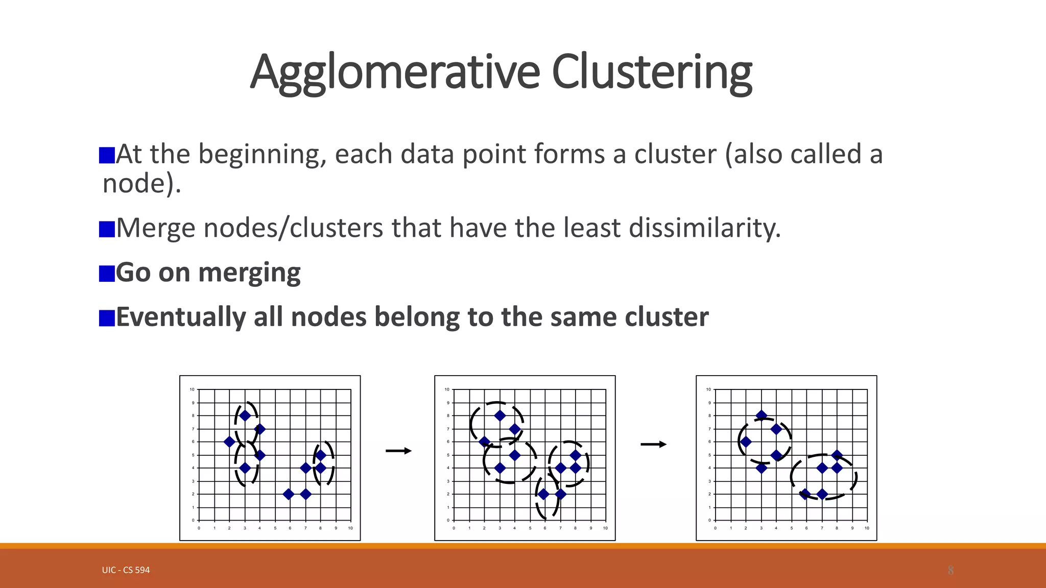
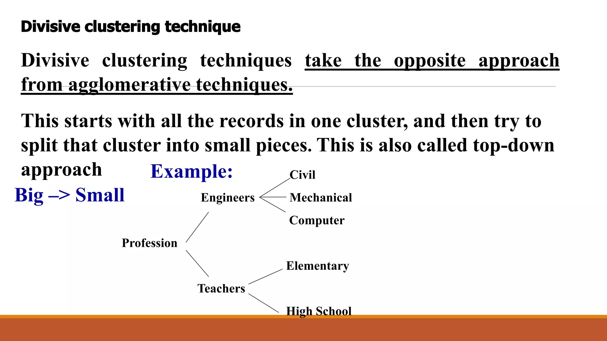
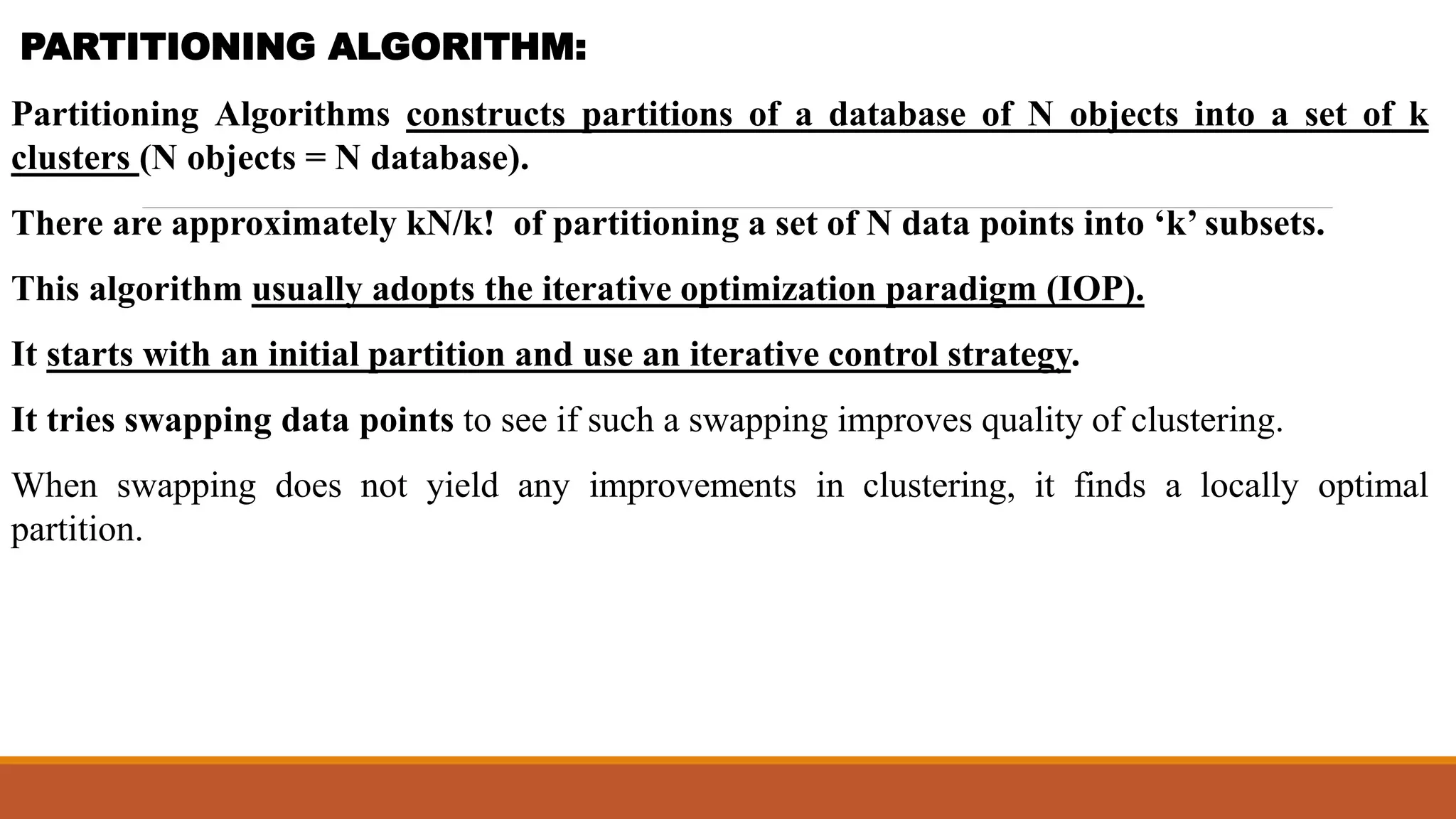
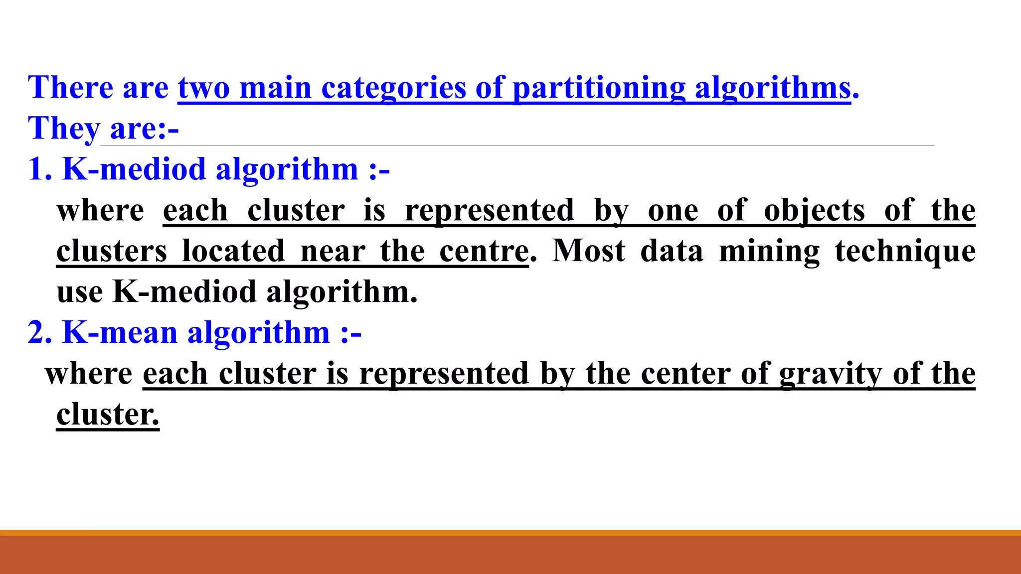
Clustering is an unsupervised machine learning technique used to group unlabeled data points. There are two main approaches: hierarchical clustering and partitioning clustering. Partitioning clustering algorithms like k-means and k-medoids attempt to partition data into k clusters by optimizing a criterion function. Hierarchical clustering creates nested clusters by merging or splitting clusters. Examples of hierarchical algorithms include agglomerative clustering, which builds clusters from bottom-up, and divisive clustering, which separates clusters from top-down. Clustering can group both numerical and categorical data.

1. CLUSTERING
REFERENCES: DATA MINING TECHNIQUES BY ARUN K. PUJARI
MRS.SOWMYA JYOTHI
SDMCBM
MANGALORE

2. Introduction:
Clustering is a useful technique for the discovery of data
distribution and patterns in the underlying data.
The goal of clustering is to discover both the dense and sparse
regions (Dense= All data are closely associated together;
Sparse= Data is tingly scattered).

3. Example:
Consider a market-basket database typically a number of
items and thus the number of attributes in such a database
is very large, while the size of an average transaction is
much smaller.
Furthermore, customers with similar buying patterns,
who belong to a single cluster, may buy a small subset of
items from a much larger set that defines the cluster.
Thus, conventional clustering methods that handle only
numerical data are not suitable for data mining purpose.

4. There are two main approaches to clustering:
Hierarchical clustering
Partitioning clustering

5. PARTITIONING CLUSTERING
The partition clustering techniques, partition the database into
predefined number of clusters.
They attempt to determine K partitions that optimize a certain
criterion function.
Partition clustering algorithms are of two types:
K- MEANS ALGORITHM
K- MEDIOD ALGORITHM
K- MODE ALGORITHM- is another type.

6. HIERARCHICAL CLUSTERING
The hierarchical clustering techniques do a sequence of
partitions, in which each partition is nested into the next
partition in the sequence. They create a hierarchy of clusters
from small to big or big to small.
The hierarchical techniques are of 2 types:
Agglomerative clustering
Divisive clustering technique

7. Agglomerative clustering techniques starts with as many clusters as
there are records, with each cluster having one record.
Then pairs of clusters are successively merged until the numbers of
clusters reduces to k. This is also called Bottom-up approach.
At each stage, the pairs of the clusters merged are the ones that are
nearest to each other.
If merging is continued, it terminates in a hierarchy of clusters which is
built with just a single cluster containing all the records, at the top of
the hierarchy.
Example: Small –> Big = Week->Month->Year

8. UIC - CS 594 8
Agglomerative Clustering
At the beginning, each data point forms a cluster (also called a
node).
Merge nodes/clusters that have the least dissimilarity.
Go on merging
Eventually all nodes belong to the same cluster
0
1
2
3
4
5
6
7
8
9
10
0 1 2 3 4 5 6 7 8 9 10
0
1
2
3
4
5
6
7
8
9
10
0 1 2 3 4 5 6 7 8 9 10
0
1
2
3
4
5
6
7
8
9
10
0 1 2 3 4 5 6 7 8 9 10

9. Divisive clustering techniques take the opposite approach
from agglomerative techniques.
This starts with all the records in one cluster, and then try to
split that cluster into small pieces. This is also called top-down
approach Example:
Big –> Small
Civil
Engineers Mechanical
Computer
Profession
Elementary
Teachers
High School

10. UIC - CS 594 10
Divisive Clustering
Inverse order of agglomerative clustering
Eventually each node forms a cluster on its own
0
1
2
3
4
5
6
7
8
9
10
0 1 2 3 4 5 6 7 8 9 10
0
1
2
3
4
5
6
7
8
9
10
0 1 2 3 4 5 6 7 8 9 10
0
1
2
3
4
5
6
7
8
9
10
0 1 2 3 4 5 6 7 8 9 10

11. Clustering can be performed on both numerical and categorical
data.
For clustering of numerical data, the inherit geometric properties
can be used to define the distance between points.
But for the clustering of categorical data such a criterion does
not exist and many data sets also consists of categorical attributes on
which distance functions are not naturally defined.

12. Some more examples are :
Quantitative:
•Weight in pounds
•Length in inches
•Time in seconds
•Number of questions correct on a quiz
Categorical
•Model of car
•Gender
•Yes or No
•Pass or Fail

13. Partitioning Algorithms constructs partitions of a database of N objects into a set of k
clusters (N objects = N database).
There are approximately kN/k! of partitioning a set of N data points into ‘k’ subsets.
This algorithm usually adopts the iterative optimization paradigm (IOP).
It starts with an initial partition and use an iterative control strategy.
It tries swapping data points to see if such a swapping improves quality of clustering.
When swapping does not yield any improvements in clustering, it finds a locally optimal
partition.

14. There are two main categories of partitioning algorithms.
They are:-
1. K-mediod algorithm :-
where each cluster is represented by one of objects of the
clusters located near the centre. Most data mining technique
use K-mediod algorithm.
2. K-mean algorithm :-
where each cluster is represented by the center of gravity of the
cluster.

15. PAM (Partition Around Medoids, 1987)
oFind representative objects, called medoids, in clusters
◦ PAM uses a k-medoid method to identify the clusters.
◦ PAM selects k objects arbitrarily from the data as medoids.
◦ Each of these k objects are representatives of k classes.
◦ It starts from an initial set of medoids and iteratively replaces one of the
medoids by one of the non-medoids, if it improves the total distance of the
resulting clustering. PAM works effectively for small data sets, but does not scale
well for large data sets

16. Partition Around Medoids (PAM)
•The algorithm starts with arbitrarily selected k-medoids and
iteratively improves upon the selection.
•In each step, a swap between a selected object Oi and a non-
selected object Oh is made, as long as such a swap results in an
improvement in the quality of clustering.
•To calculate the effect of such a swap between Oi and Oh, a cost Cih
is computed.
•The algorithm has 2 important modules
1. Partitioning of the database for a given set of mediods
2. Iterative selection of medoids.

17. Partitioning
If Oj is a non-selected object and Oi is a medoid, then we say
that Oj belongs to the cluster represented by Oi,
if d(Oi, Oj)= Min oe(Oj, Oe), where the minimum is taken
over all medoids Oe and
d(Oa, Ob) determines the distance or dissimilarity between
objects Oa and Ob.

18. CLARA: (Clustering LARge Applications)
(Kaufman & Rousseeuw 1990) reduces the computational complexity
by drawing multiple samples of the objects and applying the PAM
algorithm on each sample. CLARA accepts only the actual
measurements.
Compared to PAM, CLARA can deal with much larger data sets.
Like PAM, CLARA also finds objects that are centrally located in
the clusters.
The main problem with PAM that it
finds the entire dissimilarity matrix at a time.

19. DBSCAN:-
Density Based Spatial Clustering of Applications of Noise
Uses a density-based notion of clusters to discover clusters of arbitrary shapes.
The idea of DBSCAN is that, for each object of a cluster, the neighborhood of a
given radius has to contain at least a minimum number of data objects.
In other words, the density of the neighborhood must exceed a threshold.
The critical parameter is the distance function for the data objects.

20. Although algorithms like BIRCH, CURE, CLARANS are suitable
for large dataset. These are designed primarily for numeric data.
The important algorithms which are used for a categorical data
set are CACTUS, ROCK, STIRR.
One important common feature of these three algorithms is that they
attempt to model the similarity of categorical attributes in more or less
similar manner.

21. ROCK (Robust hierarchical-clustering with links) tries to introduce
a concept called neighbor and link.
STIRR(Sieving Through Iterated Relational Reinforcement).
CACTUS (Clustering Categorical Data Using Summaries) also makes
use of occurrences as the similarity measure.

22. STIRR(Sieving Through Iterated Relational Reinforcement)
Proposed by Gibson, Kleinberg and Raghavan, is an iterative algorithm based
on non-linear dynamical systems.
The database is represented as a graph, where each distinct value in the domain
of each attribute is represented by a weighted node. Thus, if there are N
attributes and the domain size of the ith attribute is di, then the number of
nodes in the graph is
For each tuple in the database, an edge represents a set of nodes which
participate in that tuple. Thus, a tuple is represented as a collection of nodes,
one from each attribute type. We assign a weight to each node. The set of
weights of all the nodes define the configuration of this structure. The
algorithm proceeds iteratively to update the weight of each node, based on the
weights of other nodes to which it is connected. Thus, it moves from one
configuration to the other till it reaches a stable point.