Data science related topic

1. Clustering

2. Clustering
• clustering is the process of partitioning a set of data
objects(or observations) into subsets. Clustering groups
data into sets of related observations or clusters, so that
observations within each group are more similar to other
observations within the group than to observations within
other groups.
• Clustering is an unsupervised method for grouping. By
unsupervised, we mean that the groups are not known in
advance and a goal—a specific variable—is not used to
direct how the grouping is generated. Instead, all variables
are considered in the analysis.

3. Clustering
• The clustering method chosen to subdivide
the data into groups applies an automated
procedure to discover the groups based on
some criteria and its solution is extracted from
patterns or structure existing in the data.

4. Requirements for Cluster Analysis
• Scalability: Many clustering algorithms work well on small data sets
containing fewer than several hundred data objects; however, a large database
may contain millions or even billions of objects, particularly in Web search
scenarios. Clustering on only a sample of a given large data set may lead to
biased results. Therefore, highly scalable clustering algorithms are needed.
• Ability to deal with different types of attributes: Many algorithms are designed
to cluster numeric (interval-based) data. However, applications may require
clustering other data types, such as binary, nominal (categorical), and ordinal
data, or mixtures of these data types. Recently, more and more applications
need clustering techniques for complex data types such as graphs, sequences,
images, and documents.
• Requirements for domain knowledge to determine input parameters: Many
clustering algorithms require users to provide domain knowledge in the form of
input parameters such as the desired number of clusters. Consequently, the
clustering results may be sensitive to such parameters

5. Requirements for Cluster Analysis
• Ability to deal with noisy data: Most real-world data sets contain outliers
and/or missing, unknown, or erroneous data. Sensor readings, for
example, are often noisy—some readings may be inaccurate due to the
sensing mechanisms, and some readings may be erroneous due to
interferences from surrounding transient objects.
Clustering algorithms can be sensitive to such noise and may produce
poor-quality clusters. Therefore, we need clustering methods that are
robust to noise.
• Incremental clustering and insensitivity to input order: In many
applications, incremental updates (representing newer data) may arrive at
any time. Some clustering algorithms cannot incorporate incremental
updates into existing clustering structures and, instead, have to re-
compute a new clustering from scratch. Clustering
algorithms may also be sensitive to the input data order.

6. Application
• Cluster analysis has been widely used in many
applications such as
• business intelligence,
• image pattern recognition,
• Web search,
• biology, and
• security etc.

7. Categories of clustering
• Partitioning Method
• HierarchicMethodally

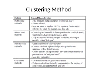
8. Clustering Methods
• Partitioning methods: Given a set of n objects, a partitioning method
constructs k partitions of the data, where each partition represents a cluster
and k <= n. That is, it divides the data into k groups such that each group
must contain at least one object. In other words, partitioning methods
conduct one-level partitioning on data sets. The basic partitioning methods
typically adopt exclusive cluster separation. That is, each object must belong
to exactly one group.
• Most partitioning methods are distance-based. Given k, the number of
partitions to construct, a partitioning method creates an initial partitioning It
then uses an iterative relocation technique that attempts to improve the
partitioning by moving objects from one group to another. The general
criterion of a good partitioning is that objects in the same cluster are “close”
or related to each other, whereas objects in different clusters are “far apart”
or very different.

9. Clustering Methods
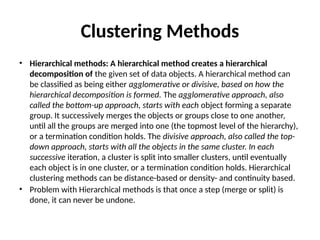
• Hierarchical methods: A hierarchical method creates a hierarchical
decomposition of the given set of data objects. A hierarchical method can
be classified as being either agglomerative or divisive, based on how the
hierarchical decomposition is formed. The agglomerative approach, also
called the bottom-up approach, starts with each object forming a separate
group. It successively merges the objects or groups close to one another,
until all the groups are merged into one (the topmost level of the hierarchy),
or a termination condition holds. The divisive approach, also called the top-
down approach, starts with all the objects in the same cluster. In each
successive iteration, a cluster is split into smaller clusters, until eventually
each object is in one cluster, or a termination condition holds. Hierarchical
clustering methods can be distance-based or density- and continuity based.
• Problem with Hierarchical methods is that once a step (merge or split) is
done, it can never be undone.

10. Clustering Method
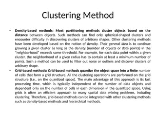
• Density-based methods: Most partitioning methods cluster objects based on the
distance between objects. Such methods can find only spherical-shaped clusters and
encounter difficulty in discovering clusters of arbitrary shapes. Other clustering methods
have been developed based on the notion of density. Their general idea is to continue
growing a given cluster as long as the density (number of objects or data points) in the
“neighborhood” exceeds some threshold. For example, for each data point within a given
cluster, the neighborhood of a given radius has to contain at least a minimum number of
points. Such a method can be used to filter out noise or outliers and discover clusters of
arbitrary shape.
• Grid-based methods: Grid-based methods quantize the object space into a finite number
of cells that form a grid structure. All the clustering operations are performed on the grid
structure (i.e., on the quantized space). The main advantage of this approach is its fast
processing time, which is typically independent of the number of data objects and
dependent only on the number of cells in each dimension in the quantized space. Using
grids is often an efficient approach to many spatial data mining problems, including
clustering. Therefore, grid-based methods can be integrated with other clustering methods
such as density-based methods and hierarchical methods.

11. Clustering Method

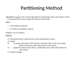
12. Partitioning Method
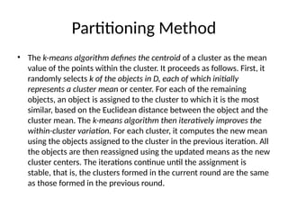
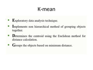
• The k-means algorithm defines the centroid of a cluster as the mean
value of the points within the cluster. It proceeds as follows. First, it
randomly selects k of the objects in D, each of which initially
represents a cluster mean or center. For each of the remaining
objects, an object is assigned to the cluster to which it is the most
similar, based on the Euclidean distance between the object and the
cluster mean. The k-means algorithm then iteratively improves the
within-cluster variation. For each cluster, it computes the new mean
using the objects assigned to the cluster in the previous iteration. All
the objects are then reassigned using the updated means as the new
cluster centers. The iterations continue until the assignment is
stable, that is, the clusters formed in the current round are the same
as those formed in the previous round.

13. Partitioning Method

14. K-mean
•

15. Steps of Clustering

16. Example

17. Example cont.

18. Example..

19. Example..

20. Example cont..

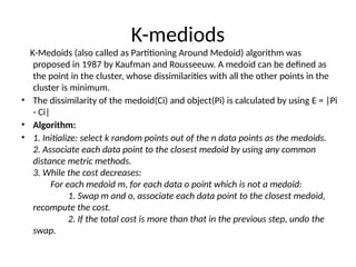
21. K-mediods
K-Medoids (also called as Partitioning Around Medoid) algorithm was
proposed in 1987 by Kaufman and Rousseeuw. A medoid can be defined as
the point in the cluster, whose dissimilarities with all the other points in the
cluster is minimum.
• The dissimilarity of the medoid(Ci) and object(Pi) is calculated by using E = |Pi
- Ci|
• Algorithm:
• 1. Initialize: select k random points out of the n data points as the medoids.
2. Associate each data point to the closest medoid by using any common
distance metric methods.
3. While the cost decreases:
For each medoid m, for each data o point which is not a medoid:
1. Swap m and o, associate each data point to the closest medoid,
recompute the cost.
2. If the total cost is more than that in the previous step, undo the
swap.

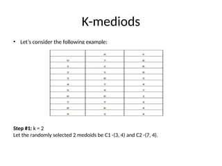
22. K-mediods
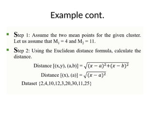
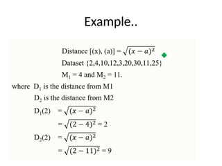
• Let’s consider the following example:
Step #1: k = 2
Let the randomly selected 2 medoids be C1 -(3, 4) and C2 -(7, 4).

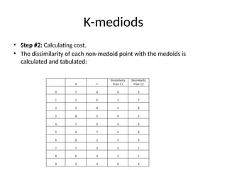
23. K-mediods
• Step #2: Calculating cost.
• The dissimilarity of each non-medoid point with the medoids is
calculated and tabulated:

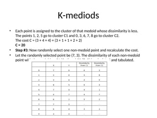
24. K-mediods
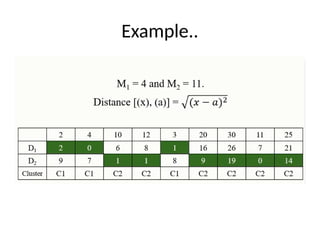
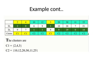
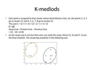
• Each point is assigned to the cluster of that medoid whose dissimilarity is less.
The points 1, 2, 5 go to cluster C1 and 0, 3, 6, 7, 8 go to cluster C2.
The cost C = (3 + 4 + 4) + (3 + 1 + 1 + 2 + 2)
C = 20
• Step #3: Now randomly select one non-medoid point and recalculate the cost.
• Let the randomly selected point be (7, 3). The dissimilarity of each non-medoid
point with the medoids – C1 (3, 4) and C2 (7, 3) is calculated and tabulated.

25. K-mediods
• Each point is assigned to that cluster whose dissimilarity is less. So, the points 1, 2, 5
go to cluster C1 and 0, 3, 6, 7, 8 go to cluster C2.
The cost C = (3 + 4 + 4) + (2 + 2 + 1 + 3 + 3)
C = 22
Swap Cost = Present Cost – Previous Cost
= 22 – 20 = 2 >0
• As the swap cost is not less than zero, we undo the swap. Hence (3, 4) and (7, 4) are
the final medoids. The clustering would be in the following way

26. Advantages and Disadvantages
• Advantages:
• It is simple to understand and easy to implement.
• K-Medoid Algorithm is fast and converges in a fixed number of steps.
• PAM is less sensitive to outliers than other partitioning algorithms.
• Disadvantages:
• The main disadvantage of K-Medoid algorithms is that it is not suitable
for clustering non-spherical (arbitrary shaped) groups of objects. This is
because it relies on minimizing the distances between the non-medoid
objects and the medoid (the cluster center) – briefly, it uses
compactness as clustering criteria instead of connectivity.
• It may obtain different results for different runs on the same dataset
because the first k medoids are chosen randomly.
•

27. Assignment
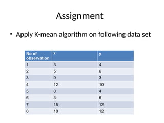
• Apply K-mean algorithm on following data set
No of
observation
x y
1 3 4
2 5 6
3 9 3
4 12 10
5 8 4
6 3 6
7 15 12
8 18 12

28. Hierarchical Methods
• Hierarchical clustering method works by grouping data
objects into a hierarchy or “tree” of clusters.
• Hierarchical clustering methods can encounter difficulties
regarding the selection of merge or split points. Such a
decision is critical, because once a group of objects is
merged or split, the process at the next step will operate
on the newly generated clusters.
• It will neither undo what was done previously, nor
perform object swapping between clusters. Thus, merge
or split decisions, if not well chosen, may lead to low-
quality clusters.

29. Hierarchical Clustering
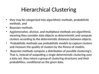
• they may be categorized into algorithmic methods, probabilistic
methods, and
• Bayesian methods.
• Agglomerative, divisive, and multiphase methods are algorithmic,
meaning they consider data objects as deterministic and compute
clusters according to the deterministic distances between objects.
• Probabilistic methods use probabilistic models to capture clusters
and measure the quality of clusters by the fitness of models.
• Bayesian methods compute a distribution of possible clustering's.
That is, instead of outputting a single deterministic clustering over
a data set, they return a group of clustering structures and their
probabilities, conditional on the given data.

30. Agglomerative versus Divisive Hierarchical
Clustering
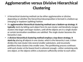
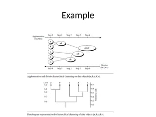
• A hierarchical clustering method can be either agglomerative or divisive,
depending on whether the hierarchical decomposition is formed in a bottom-up
(merging) or topdown (splitting) fashion
• An agglomerative hierarchical clustering method uses a bottom-up strategy. It
typically starts by letting each object form its own cluster and iteratively merges
clusters into larger and larger clusters, until all the objects are in a single cluster
or certain termination conditions are satisfied. The single cluster becomes the
hierarchy’s root.
• A divisive hierarchical clustering method employs a top-down strategy. It
starts by placing all objects in one cluster, which is the hierarchy’s root. It then
divides the root cluster into several smaller subclusters, and recursively
partitions those clusters into smaller ones. The partitioning process continues
until each cluster at the lowest level is coherent enough—either containing only
one object, or the objects within a clusterare sufficiently similar to each other.

31. Example

32. Distance Measures in Algorithmic Methods
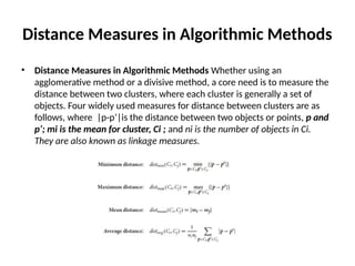
• Distance Measures in Algorithmic Methods Whether using an
agglomerative method or a divisive method, a core need is to measure the
distance between two clusters, where each cluster is generally a set of
objects. Four widely used measures for distance between clusters are as
follows, where |p-p’|is the distance between two objects or points, p and
p’; mi is the mean for cluster, Ci ; and ni is the number of objects in Ci.
They are also known as linkage measures.

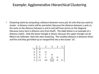
33. Example: Agglomerative Hierarchical Clustering
• Clustering starts by computing a distance between every pair of units that you want to
cluster. A distance matrix will be symmetric (because the distance between x and y is
the same as the distance between y and x) and will have zeroes on the diagonal
(because every item is distance zero from itself). The table below is an example of a
distance matrix. Only the lower triangle is shown, because the upper triangle can be
filled in by reflection. Now lets start clustering. The smallest distance is between three
and five and they get linked up or merged first into a the cluster '35'.

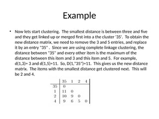
34. Example
• Now lets start clustering. The smallest distance is between three and five
and they get linked up or merged first into a the cluster '35'. To obtain the
new distance matrix, we need to remove the 3 and 5 entries, and replace
it by an entry "35" . Since we are using complete linkage clustering, the
distance between "35" and every other item is the maximum of the
distance between this item and 3 and this item and 5. For example,
d(1,3)= 3 and d(1,5)=11. So, D(1,"35")=11. This gives us the new distance
matrix. The items with the smallest distance get clustered next. This will
be 2 and 4.

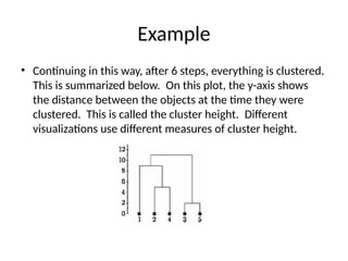
35. Example
• Continuing in this way, after 6 steps, everything is clustered.
This is summarized below. On this plot, the y-axis shows
the distance between the objects at the time they were
clustered. This is called the cluster height. Different
visualizations use different measures of cluster height.

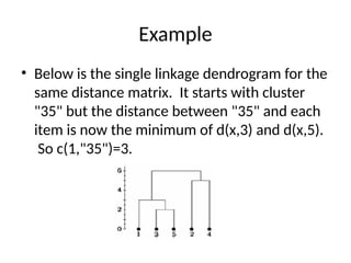
36. Example
• Below is the single linkage dendrogram for the
same distance matrix. It starts with cluster
"35" but the distance between "35" and each
item is now the minimum of d(x,3) and d(x,5).
So c(1,"35")=3.

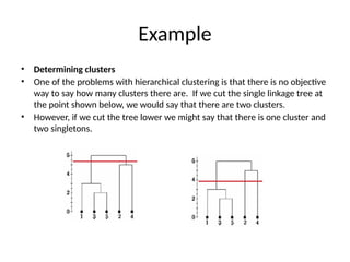
37. Example
• Determining clusters
• One of the problems with hierarchical clustering is that there is no objective
way to say how many clusters there are. If we cut the single linkage tree at
the point shown below, we would say that there are two clusters.
• However, if we cut the tree lower we might say that there is one cluster and
two singletons.