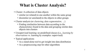
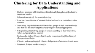
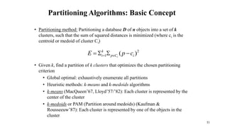
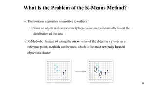
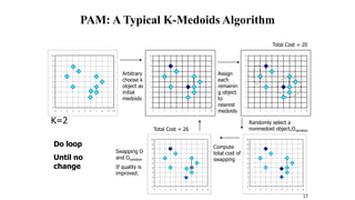
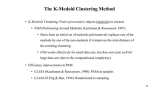
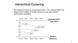
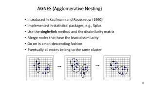
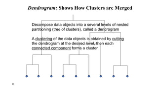
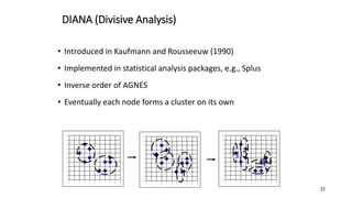
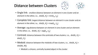
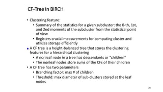
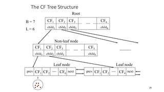
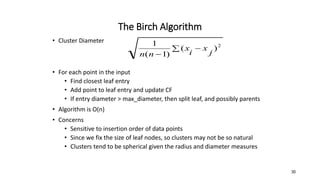
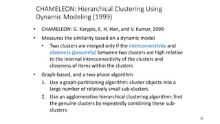
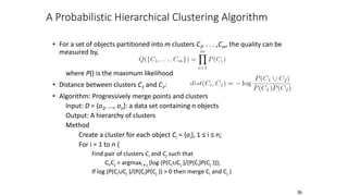
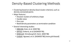
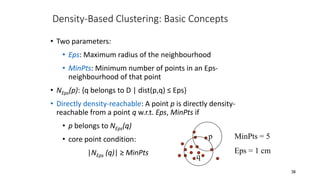
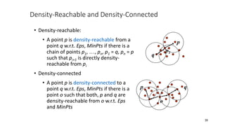
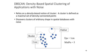
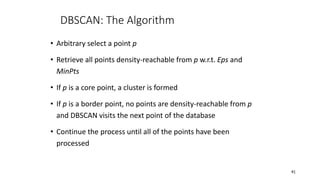
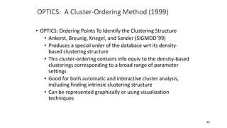
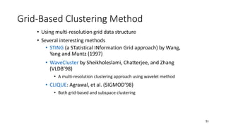
SlideShare a Scribd company logo
1 of 72
DATA MINING
TECHNIQUES
UNIT-V
2
What is Cluster Analysis?
• Cluster: A collection of data objects
• similar (or related) to one another within the same group
• dissimilar (or unrelated) to the objects in other groups
• Cluster analysis (or clustering, data segmentation, …)
• Finding similarities between data according to the
characteristics found in the data and grouping similar data
objects into clusters
• Unsupervised learning: no predefined classes (i.e., learning by
observations vs. learning by examples: supervised)
• Typical applications
• As a stand-alone tool to get insight into data distribution
• As a preprocessing step for other algorithms
3
Clustering for Data Understanding and
Applications
• Biology: taxonomy of living things: kingdom, phylum, class, order, family,
genus and species
• Information retrieval: document clustering
• Land use: Identification of areas of similar land use in an earth observation
database
• Marketing: Help marketers discover distinct groups in their customer bases,
and then use this knowledge to develop targeted marketing programs
• City-planning: Identifying groups of houses according to their house type,
value, and geographical location
• Earth-quake studies: Observed earth quake epicenters should be clustered
along continent faults
• Climate: understanding earth climate, find patterns of atmospheric and ocean
• Economic Science: market research
4
Clustering as a Preprocessing Tool (Utility)
• Summarization:
• Preprocessing for regression, PCA, classification, and
association analysis
• Compression:
• Image processing: vector quantization
• Finding K-nearest Neighbors
• Localizing search to one or a small number of clusters
• Outlier detection
• Outliers are often viewed as those “far away” from any cluster
Quality: What Is Good
Clustering?
• A good clustering method will produce high quality clusters
• high intra-class similarity: cohesive within clusters
• low inter-class similarity: distinctive between clusters
• The quality of a clustering method depends on
• the similarity measure used by the method
• its implementation, and
• Its ability to discover some or all of the hidden patterns
5
Measure the Quality of Clustering
• Dissimilarity/Similarity metric
• Similarity is expressed in terms of a distance function,
typically metric: d(i, j)
• The definitions of distance functions are usually rather
different for interval-scaled, boolean, categorical, ordinal
ratio, and vector variables
• Weights should be associated with different variables based
on applications and data semantics
• Quality of clustering:
• There is usually a separate “quality” function that measures
the “goodness” of a cluster.
• It is hard to define “similar enough” or “good enough”
• The answer is typically highly subjective
6
Considerations for Cluster Analysis
• Partitioning criteria
• Single level vs. hierarchical partitioning (often, multi-level hierarchical partitioning is
desirable)
• Separation of clusters
• Exclusive (e.g., one customer belongs to only one region) vs. non-exclusive (e.g., one
document may belong to more than one class)
• Similarity measure
• Distance-based (e.g., Euclidian, road network, vector) vs. connectivity-based (e.g., density or
contiguity)
• Clustering space
• Full space (often when low dimensional) vs. subspaces (often in high-dimensional clustering)
7
Requirements and Challenges
• Scalability
• Clustering all the data instead of only on samples
• Ability to deal with different types of attributes
• Numerical, binary, categorical, ordinal, linked, and mixture of these
• Constraint-based clustering
• User may give inputs on constraints
• Use domain knowledge to determine input parameters
• Interpretability and usability
• Others
• Discovery of clusters with arbitrary shape
• Ability to deal with noisy data
• Incremental clustering and insensitivity to input order
• High dimensionality
8
Major Clustering Approaches (I)
• Partitioning approach:
• Construct various partitions and then evaluate them by some criterion, e.g.,
minimizing the sum of square errors
• Typical methods: k-means, k-medoids, CLARANS
• Hierarchical approach:
• Create a hierarchical decomposition of the set of data (or objects) using
some criterion
• Typical methods: Diana, Agnes, BIRCH, CAMELEON
• Density-based approach:
• Based on connectivity and density functions
• Typical methods: DBSACN, OPTICS, DenClue
• Grid-based approach:
• based on a multiple-level granularity structure
• Typical methods: STING, WaveCluster, CLIQUE
9
Major Clustering Approaches (II)
• Model-based:
• A model is hypothesized for each of the clusters and tries to find the best
fit of that model to each other
• Typical methods: EM, SOM, COBWEB
• Frequent pattern-based:
• Based on the analysis of frequent patterns
• Typical methods: p-Cluster
• User-guided or constraint-based:
• Clustering by considering user-specified or application-specific constraints
• Typical methods: COD (obstacles), constrained clustering
• Link-based clustering:
• Objects are often linked together in various ways
• Massive links can be used to cluster objects: SimRank, LinkClus
10
Partitioning Algorithms: Basic Concept
• Partitioning method: Partitioning a database D of n objects into a set of k
clusters, such that the sum of squared distances is minimized (where ci is the
centroid or medoid of cluster Ci)
• Given k, find a partition of k clusters that optimizes the chosen partitioning
criterion
• Global optimal: exhaustively enumerate all partitions
• Heuristic methods: k-means and k-medoids algorithms
• k-means (MacQueen’67, Lloyd’57/’82): Each cluster is represented by the
center of the cluster
• k-medoids or PAM (Partition around medoids) (Kaufman &
Rousseeuw’87): Each cluster is represented by one of the objects in the
cluster
2
1 )
( i
C
p
k
i c
p
E i



 

11
The K-Means Clustering Method
• Given k, the k-means algorithm is implemented in four
steps:
• Partition objects into k nonempty subsets
• Compute seed points as the centroids of the clusters of
the current partitioning (the centroid is the center, i.e.,
mean point, of the cluster)
• Assign each object to the cluster with the nearest seed
point
• Go back to Step 2, stop when the assignment does not
change
12
An Example of K-Means Clustering
K=2
Arbitrarily
partition
objects into
k groups
Update the
cluster
centroids
Update the
cluster
centroids
Reassign objects
Loop if
needed
13
The initial data set
 Partition objects into k nonempty
subsets
 Repeat
 Compute centroid (i.e., mean
point) for each partition
 Assign each object to the
cluster of its nearest centroid
 Until no change
Comments on the K-Means Method
• Strength: Efficient: O(tkn), where n is # objects, k is # clusters, and t is #
iterations. Normally, k, t << n.
• Comparing: PAM: O(k(n-k)2 ), CLARA: O(ks2 + k(n-k))
• Comment: Often terminates at a local optimal.
• Weakness
• Applicable only to objects in a continuous n-dimensional space
• Using the k-modes method for categorical data
• In comparison, k-medoids can be applied to a wide range of data
• Need to specify k, the number of clusters, in advance (there are ways to
automatically determine the best k (see Hastie et al., 2009)
• Sensitive to noisy data and outliers
• Not suitable to discover clusters with non-convex shapes
14
Variations of the K-Means Method
• Most of the variants of the k-means which differ in
• Selection of the initial k means
• Dissimilarity calculations
• Strategies to calculate cluster means
• Handling categorical data: k-modes
• Replacing means of clusters with modes
• Using new dissimilarity measures to deal with categorical objects
• Using a frequency-based method to update modes of clusters
• A mixture of categorical and numerical data: k-prototype method
15
What Is the Problem of the K-Means Method?
• The k-means algorithm is sensitive to outliers !
• Since an object with an extremely large value may substantially distort the
distribution of the data
• K-Medoids: Instead of taking the mean value of the object in a cluster as a
reference point, medoids can be used, which is the most centrally located
object in a cluster
0
1
2
3
4
5
6
7
8
9
10
0 1 2 3 4 5 6 7 8 9 10
0
1
2
3
4
5
6
7
8
9
10
0 1 2 3 4 5 6 7 8 9 10
16
17
PAM: A Typical K-Medoids Algorithm
0
1
2
3
4
5
6
7
8
9
10
0 1 2 3 4 5 6 7 8 9 10
Total Cost = 20
0
1
2
3
4
5
6
7
8
9
10
0 1 2 3 4 5 6 7 8 9 10
K=2
Arbitrary
choose k
object as
initial
medoids
0
1
2
3
4
5
6
7
8
9
10
0 1 2 3 4 5 6 7 8 9 10
Assign
each
remainin
g object
to
nearest
medoids
Randomly select a
nonmedoid object,Oramdom
Compute
total cost of
swapping
0
1
2
3
4
5
6
7
8
9
10
0 1 2 3 4 5 6 7 8 9 10
Total Cost = 26
Swapping O
and Oramdom
If quality is
improved.
Do loop
Until no
change
0
1
2
3
4
5
6
7
8
9
10
0 1 2 3 4 5 6 7 8 9 10
The K-Medoid Clustering Method
• K-Medoids Clustering: Find representative objects (medoids) in clusters
• PAM (Partitioning Around Medoids, Kaufmann & Rousseeuw 1987)
• Starts from an initial set of medoids and iteratively replaces one of the
medoids by one of the non-medoids if it improves the total distance of
the resulting clustering
• PAM works effectively for small data sets, but does not scale well for
large data sets (due to the computational complexity)
• Efficiency improvement on PAM
• CLARA (Kaufmann & Rousseeuw, 1990): PAM on samples
• CLARANS (Ng & Han, 1994): Randomized re-sampling
18
Hierarchical Clustering
• Use distance matrix as clustering criteria. This method does not
require the number of clusters k as an input, but needs a
termination condition
Step 0 Step 1 Step 2 Step 3 Step 4
b
d
c
e
a
a b
d e
c d e
a b c d e
Step 4 Step 3 Step 2 Step 1 Step 0
agglomerative
(AGNES)
divisive
(DIANA)
19
AGNES (Agglomerative Nesting)
• Introduced in Kaufmann and Rousseeuw (1990)
• Implemented in statistical packages, e.g., Splus
• Use the single-link method and the dissimilarity matrix
• Merge nodes that have the least dissimilarity
• Go on in a non-descending fashion
• Eventually all nodes belong to the same cluster
0
1
2
3
4
5
6
7
8
9
10
0 1 2 3 4 5 6 7 8 9 10
0
1
2
3
4
5
6
7
8
9
10
0 1 2 3 4 5 6 7 8 9 10
0
1
2
3
4
5
6
7
8
9
10
0 1 2 3 4 5 6 7 8 9 10
20
Dendrogram: Shows How Clusters are Merged
Decompose data objects into a several levels of nested
partitioning (tree of clusters), called a dendrogram
A clustering of the data objects is obtained by cutting
the dendrogram at the desired level, then each
connected component forms a cluster
21
DIANA (Divisive Analysis)
• Introduced in Kaufmann and Rousseeuw (1990)
• Implemented in statistical analysis packages, e.g., Splus
• Inverse order of AGNES
• Eventually each node forms a cluster on its own
0
1
2
3
4
5
6
7
8
9
10
0 1 2 3 4 5 6 7 8 9 10
0
1
2
3
4
5
6
7
8
9
10
0 1 2 3 4 5 6 7 8 9 10
0
1
2
3
4
5
6
7
8
9
10
0 1 2 3 4 5 6 7 8 9 10
22
Distance between Clusters
• Single link: smallest distance between an element in one cluster and an
element in the other, i.e., dist(Ki, Kj) = min(tip, tjq)
• Complete link: largest distance between an element in one cluster and an
element in the other, i.e., dist(Ki, Kj) = max(tip, tjq)
• Average: avg distance between an element in one cluster and an element
in the other, i.e., dist(Ki, Kj) = avg(tip, tjq)
• Centroid: distance between the centroids of two clusters, i.e., dist(Ki, Kj) =
dist(Ci, Cj)
• Medoid: distance between the medoids of two clusters, i.e., dist(Ki, Kj) =
dist(Mi, Mj)
• Medoid: a chosen, centrally located object in the cluster
X X
23
Centroid, Radius and Diameter of a Cluster (for numerical data
sets)
• Centroid: the “middle” of a cluster
• Radius: square root of average distance from any point of the
cluster to its centroid
• Diameter: square root of average mean squared distance
between all pairs of points in the cluster
N
t
N
i ip
m
C
)
(
1



N
m
c
ip
t
N
i
m
R
2
)
(
1




)
1
(
2
)
(
1
1







N
N
iq
t
ip
t
N
i
N
i
m
D
24
Extensions to Hierarchical Clustering
• Major weakness of agglomerative clustering methods
• Can never undo what was done previously
• Do not scale well: time complexity of at least O(n2), where n is
the number of total objects
• Integration of hierarchical & distance-based clustering
• BIRCH (1996): uses CF-tree and incrementally adjusts the
quality of sub-clusters
• CHAMELEON (1999): hierarchical clustering using dynamic
modeling
25
BIRCH (Balanced Iterative Reducing and
Clustering Using Hierarchies)
• Zhang, Ramakrishnan & Livny, SIGMOD’96
• Incrementally construct a CF (Clustering Feature) tree, a hierarchical data
structure for multiphase clustering
• Phase 1: scan DB to build an initial in-memory CF tree (a multi-level
compression of the data that tries to preserve the inherent clustering
structure of the data)
• Phase 2: use an arbitrary clustering algorithm to cluster the leaf nodes of
the CF-tree
• Scales linearly: finds a good clustering with a single scan and improves the
quality with a few additional scans
• Weakness: handles only numeric data, and sensitive to the order of the data
record
26
Clustering Feature Vector in BIRCH
Clustering Feature (CF): CF = (N, LS, SS)
N: Number of data points
LS: linear sum of N points:
SS: square sum of N points
0
1
2
3
4
5
6
7
8
9
10
0 1 2 3 4 5 6 7 8 9 10
CF = (5, (16,30),(54,190))
(3,4)
(2,6)
(4,5)
(4,7)
(3,8)


N
i
i
X
1
2
1


N
i
i
X
27
CF-Tree in BIRCH
• Clustering feature:
• Summary of the statistics for a given subcluster: the 0-th, 1st,
and 2nd moments of the subcluster from the statistical point
of view
• Registers crucial measurements for computing cluster and
utilizes storage efficiently
A CF tree is a height-balanced tree that stores the clustering
features for a hierarchical clustering
• A nonleaf node in a tree has descendants or “children”
• The nonleaf nodes store sums of the CFs of their children
• A CF tree has two parameters
• Branching factor: max # of children
• Threshold: max diameter of sub-clusters stored at the leaf
nodes
28
The CF Tree Structure
CF1
child1
CF3
child3
CF2
child2
CF6
child6
CF1
child1
CF3
child3
CF2
child2
CF5
child5
CF1 CF2 CF6
prev next CF1 CF2 CF4
prev next
B = 7
L = 6
Root
Non-leaf node
Leaf node Leaf node
29
The Birch Algorithm
• Cluster Diameter
• For each point in the input
• Find closest leaf entry
• Add point to leaf entry and update CF
• If entry diameter > max_diameter, then split leaf, and possibly parents
• Algorithm is O(n)
• Concerns
• Sensitive to insertion order of data points
• Since we fix the size of leaf nodes, so clusters may not be so natural
• Clusters tend to be spherical given the radius and diameter measures
 

2
)
(
)
1
(
1
j
x
i
x
n
n
30
CHAMELEON: Hierarchical Clustering Using
Dynamic Modeling (1999)
• CHAMELEON: G. Karypis, E. H. Han, and V. Kumar, 1999
• Measures the similarity based on a dynamic model
• Two clusters are merged only if the interconnectivity and
closeness (proximity) between two clusters are high relative
to the internal interconnectivity of the clusters and
closeness of items within the clusters
• Graph-based, and a two-phase algorithm
1. Use a graph-partitioning algorithm: cluster objects into a
large number of relatively small sub-clusters
2. Use an agglomerative hierarchical clustering algorithm: find
the genuine clusters by repeatedly combining these sub-
clusters
31
Overall Framework of CHAMELEON
Construct (K-NN)
Sparse Graph Partition the Graph
Merge Partition
Final Clusters
Data Set
K-NN Graph
P and q are connected if
q is among the top k
closest neighbors of p
Relative interconnectivity:
connectivity of c1 and c2
over internal connectivity
Relative closeness:
closeness of c1 and c2 over
internal closeness 32
33
CHAMELEON (Clustering Complex Objects)
Probabilistic Hierarchical Clustering
• Algorithmic hierarchical clustering
• Nontrivial to choose a good distance measure
• Hard to handle missing attribute values
• Optimization goal not clear: heuristic, local search
• Probabilistic hierarchical clustering
• Use probabilistic models to measure distances between clusters
• Generative model: Regard the set of data objects to be clustered as a
sample of the underlying data generation mechanism to be analyzed
• Easy to understand, same efficiency as algorithmic agglomerative
clustering method, can handle partially observed data
• In practice, assume the generative models adopt common distributions
functions, e.g., Gaussian distribution or Bernoulli distribution, governed by
parameters
34
Generative Model
• Given a set of 1-D points X = {x1, …, xn} for clustering analysis
& assuming they are generated by a Gaussian distribution:
• The probability that a point xi ∈ X is generated by the model
• The likelihood that X is generated by the model:
• The task of learning the generative model: find the
parameters μ and σ2 such that
the maximum likelihood
35
A Probabilistic Hierarchical Clustering Algorithm
• For a set of objects partitioned into m clusters C1, . . . ,Cm, the quality can be
measured by,
where P() is the maximum likelihood
• Distance between clusters C1 and C2:
• Algorithm: Progressively merge points and clusters
Input: D = {o1, ..., on}: a data set containing n objects
Output: A hierarchy of clusters
Method
Create a cluster for each object Ci = {oi}, 1 ≤ i ≤ n;
For i = 1 to n {
Find pair of clusters Ci and Cj such that
Ci,Cj = argmaxi ≠ j {log (P(Ci∪Cj )/(P(Ci)P(Cj ))};
If log (P(Ci∪Cj )/(P(Ci)P(Cj )) > 0 then merge Ci and Cj }
36
Density-Based Clustering Methods
• Clustering based on density (local cluster criterion), such as
density-connected points
• Major features:
• Discover clusters of arbitrary shape
• Handle noise
• One scan
• Need density parameters as termination condition
• Several interesting studies:
• DBSCAN: Ester, et al. (KDD’96)
• OPTICS: Ankerst, et al (SIGMOD’99).
• DENCLUE: Hinneburg & D. Keim (KDD’98)
• CLIQUE: Agrawal, et al. (SIGMOD’98) (more grid-based)
37
Density-Based Clustering: Basic Concepts
• Two parameters:
• Eps: Maximum radius of the neighbourhood
• MinPts: Minimum number of points in an Eps-
neighbourhood of that point
• NEps(p): {q belongs to D | dist(p,q) ≤ Eps}
• Directly density-reachable: A point p is directly density-
reachable from a point q w.r.t. Eps, MinPts if
• p belongs to NEps(q)
• core point condition:
|NEps (q)| ≥ MinPts
MinPts = 5
Eps = 1 cm
p
q
38
Density-Reachable and Density-Connected
• Density-reachable:
• A point p is density-reachable from a
point q w.r.t. Eps, MinPts if there is a
chain of points p1, …, pn, p1 = q, pn = p
such that pi+1 is directly density-
reachable from pi
• Density-connected
• A point p is density-connected to a
point q w.r.t. Eps, MinPts if there is a
point o such that both, p and q are
density-reachable from o w.r.t. Eps
and MinPts
p
q
p1
p q
o
39
DBSCAN: Density-Based Spatial Clustering of
Applications with Noise
• Relies on a density-based notion of cluster: A cluster is defined as
a maximal set of density-connected points
• Discovers clusters of arbitrary shape in spatial databases with
noise
Core
Border
Outlier
Eps = 1cm
MinPts = 5
40
DBSCAN: The Algorithm
• Arbitrary select a point p
• Retrieve all points density-reachable from p w.r.t. Eps and
MinPts
• If p is a core point, a cluster is formed
• If p is a border point, no points are density-reachable from p
and DBSCAN visits the next point of the database
• Continue the process until all of the points have been
processed
41
DBSCAN: Sensitive to Parameters
42
OPTICS: A Cluster-Ordering Method (1999)
• OPTICS: Ordering Points To Identify the Clustering Structure
• Ankerst, Breunig, Kriegel, and Sander (SIGMOD’99)
• Produces a special order of the database wrt its density-
based clustering structure
• This cluster-ordering contains info equiv to the density-based
clusterings corresponding to a broad range of parameter
settings
• Good for both automatic and interactive cluster analysis,
including finding intrinsic clustering structure
• Can be represented graphically or using visualization
techniques
43
OPTICS: Some Extension from DBSCAN
• Index-based:
• k = number of dimensions
• N = 20
• p = 75%
• M = N(1-p) = 5
• Complexity: O(NlogN)
• Core Distance:
• min eps s.t. point is core
• Reachability Distance
D
p2
MinPts = 5
e = 3 cm
Max (core-distance (o), d (o, p))
r(p1, o) = 2.8cm. r(p2,o) = 4cm
o
o
p1
44
e
e
Reachability
-distance
Cluster-order
of the objects
undefined
e‘
45
46
Density-Based Clustering: OPTICS & Its Applications
DENCLUE: Using Statistical Density Functions
• DENsity-based CLUstEring by Hinneburg & Keim (KDD’98)
• Using statistical density functions:
• Major features
• Solid mathematical foundation
• Good for data sets with large amounts of noise
• Allows a compact mathematical description of arbitrarily shaped clusters
in high-dimensional data sets
• Significant faster than existing algorithm (e.g., DBSCAN)
• But needs a large number of parameters
f x y e
Gaussian
d x y
( , )
( , )


2
2
2  


N
i
x
x
d
D
Gaussian
i
e
x
f 1
2
)
,
(
2
2
)
( 






N
i
x
x
d
i
i
D
Gaussian
i
e
x
x
x
x
f 1
2
)
,
(
2
2
)
(
)
,
( 
influence of y
on x
total influence
on x
gradient of x in
the direction of
xi
47
• Uses grid cells but only keeps information about grid cells that do actually
contain data points and manages these cells in a tree-based access structure
• Influence function: describes the impact of a data point within its
neighborhood
• Overall density of the data space can be calculated as the sum of the influence
function of all data points
• Clusters can be determined mathematically by identifying density attractors
• Density attractors are local maximal of the overall density function
• Center defined clusters: assign to each density attractor the points density
attracted to it
• Arbitrary shaped cluster: merge density attractors that are connected through
paths of high density (> threshold)
Denclue: Technical Essence
48
Density Attractor
49
Center-Defined and Arbitrary
50
Grid-Based Clustering Method
• Using multi-resolution grid data structure
• Several interesting methods
• STING (a STatistical INformation Grid approach) by Wang,
Yang and Muntz (1997)
• WaveCluster by Sheikholeslami, Chatterjee, and Zhang
(VLDB’98)
• A multi-resolution clustering approach using wavelet method
• CLIQUE: Agrawal, et al. (SIGMOD’98)
• Both grid-based and subspace clustering
51
STING: A Statistical Information Grid Approach
• Wang, Yang and Muntz (VLDB’97)
• The spatial area is divided into rectangular cells
• There are several levels of cells corresponding to different levels of
resolution
52
The STING Clustering Method
• Each cell at a high level is partitioned into a number of smaller
cells in the next lower level
• Statistical info of each cell is calculated and stored beforehand
and is used to answer queries
• Parameters of higher level cells can be easily calculated from
parameters of lower level cell
• count, mean, s, min, max
• type of distribution—normal, uniform, etc.
• Use a top-down approach to answer spatial data queries
• Start from a pre-selected layer—typically with a small number of
cells
• For each cell in the current level compute the confidence interval
53
STING Algorithm and Its Analysis
• Remove the irrelevant cells from further consideration
• When finish examining the current layer, proceed to the next
lower level
• Repeat this process until the bottom layer is reached
• Advantages:
• Query-independent, easy to parallelize, incremental update
• O(K), where K is the number of grid cells at the lowest level
• Disadvantages:
• All the cluster boundaries are either horizontal or vertical,
and no diagonal boundary is detected
54
55
CLIQUE (Clustering In QUEst)
• Agrawal, Gehrke, Gunopulos, Raghavan (SIGMOD’98)
• Automatically identifying subspaces of a high dimensional data space that allow
better clustering than original space
• CLIQUE can be considered as both density-based and grid-based
• It partitions each dimension into the same number of equal length interval
• It partitions an m-dimensional data space into non-overlapping rectangular
units
• A unit is dense if the fraction of total data points contained in the unit
exceeds the input model parameter
• A cluster is a maximal set of connected dense units within a subspace
56
CLIQUE: The Major Steps
• Partition the data space and find the number of points that lie
inside each cell of the partition.
• Identify the subspaces that contain clusters using the Apriori
principle
• Identify clusters
• Determine dense units in all subspaces of interests
• Determine connected dense units in all subspaces of interests.
• Generate minimal description for the clusters
• Determine maximal regions that cover a cluster of connected
dense units for each cluster
• Determination of minimal cover for each cluster
57
Salary
(10,000)
20 30 40 50 60
age
5
4
3
1
2
6
7
0
20 30 40 50 60
age
5
4
3
1
2
6
7
0
Vacation
(week)
age
Vacation
30 50
 = 3
58
Strength and Weakness of CLIQUE
• Strength
• automatically finds subspaces of the highest dimensionality
such that high density clusters exist in those subspaces
• insensitive to the order of records in input and does not
presume some canonical data distribution
• scales linearly with the size of input and has good scalability
as the number of dimensions in the data increases
• Weakness
• The accuracy of the clustering result may be degraded at the
expense of simplicity of the method
Evaluation of clustering-Assessing Clustering Tendency
• Assess if non-random structure exists in the data by measuring the probability that the data is
generated by a uniform data distribution
• Test spatial randomness by statistic test: Hopkins Static
• Given a dataset D regarded as a sample of a random variable o, determine how far away o is
from being uniformly distributed in the data space
• Sample n points, p1, …, pn, uniformly from D. For each pi, find its nearest neighbor in D: xi =
min{dist (pi, v)} where v in D
• Sample n points, q1, …, qn, uniformly from D. For each qi, find its nearest neighbor in D – {qi}:
yi = min{dist (qi, v)} where v in D and v ≠ qi
• Calculate the Hopkins Statistic:
• If D is uniformly distributed, ∑ xi and ∑ yi will be close to each other and H is close to 0.5. If D
is highly skewed, H is close to 0
59
Determine the Number of Clusters
• Empirical method
• # of clusters ≈√n/2 for a dataset of n points
• Elbow method
• Use the turning point in the curve of sum of within cluster variance w.r.t
the # of clusters
• Cross validation method
• Divide a given data set into m parts
• Use m – 1 parts to obtain a clustering model
• Use the remaining part to test the quality of the clustering
• E.g., For each point in the test set, find the closest centroid, and use
the sum of squared distance between all points in the test set and the
closest centroids to measure how well the model fits the test set
• For any k > 0, repeat it m times, compare the overall quality measure w.r.t.
different k’s, and find # of clusters that fits the data the best
60
Measuring Clustering Quality
• Two methods: extrinsic vs. intrinsic
• Extrinsic: supervised, i.e., the ground truth is available
• Compare a clustering against the ground truth using certain
clustering quality measure
• Ex. BCubed precision and recall metrics
• Intrinsic: unsupervised, i.e., the ground truth is unavailable
• Evaluate the goodness of a clustering by considering how well
the clusters are separated, and how compact the clusters are
• Ex. Silhouette coefficient
61
Measuring Clustering Quality: Extrinsic Methods
• Clustering quality measure: Q(C, Cg), for a clustering C given the ground truth Cg.
• Q is good if it satisfies the following 4 essential criteria
• Cluster homogeneity: the purer, the better
• Cluster completeness: should assign objects belong to the same category in
the ground truth to the same cluster
• Rag bag: putting a heterogeneous object into a pure cluster should be
penalized more than putting it into a rag bag (i.e., “miscellaneous” or “other”
category)
• Small cluster preservation: splitting a small category into pieces is more
harmful than splitting a large category into pieces
62
63
What Are Outliers?
• Outlier: A data object that deviates significantly from the normal objects as if it were generated
by a different mechanism
• Ex.: Unusual credit card purchase, sports: Michael Jordon, Wayne Gretzky, ...
• Outliers are different from the noise data
• Noise is random error or variance in a measured variable
• Noise should be removed before outlier detection
• Outliers are interesting: It violates the mechanism that generates the normal data
• Outlier detection vs. novelty detection: early stage, outlier; but later merged into the model
• Applications:
• Credit card fraud detection
• Telecom fraud detection
• Customer segmentation
• Medical analysis
64
Types of Outliers (I)
• Three kinds: global, contextual and collective outliers
• Global outlier (or point anomaly)
• Object is Og if it significantly deviates from the rest of the data set
• Ex. Intrusion detection in computer networks
• Issue: Find an appropriate measurement of deviation
• Contextual outlier (or conditional outlier)
• Object is Oc if it deviates significantly based on a selected context
• Ex. 80o F in Urbana: outlier? (depending on summer or winter?)
• Attributes of data objects should be divided into two groups
• Contextual attributes: defines the context, e.g., time & location
• Behavioral attributes: characteristics of the object, used in outlier
evaluation, e.g., temperature
• Can be viewed as a generalization of local outliers—whose density
significantly deviates from its local area
• Issue: How to define or formulate meaningful context?
Global Outlier
65
Types of Outliers (II)
• Collective Outliers
• A subset of data objects collectively deviate significantly
from the whole data set, even if the individual data objects
may not be outliers
• Applications: E.g., intrusion detection:
• When a number of computers keep sending denial-of-
service packages to each other
Collective Outlier
 Detection of collective outliers
 Consider not only behavior of individual objects, but also that of
groups of objects
 Need to have the background knowledge on the relationship
among data objects, such as a distance or similarity measure
on objects.
 A data set may have multiple types of outlier
 One object may belong to more than one type of outlier
66
Challenges of Outlier Detection
 Modeling normal objects and outliers properly
 Hard to enumerate all possible normal behaviors in an application
 The border between normal and outlier objects is often a gray area
 Application-specific outlier detection
 Choice of distance measure among objects and the model of
relationship among objects are often application-dependent
 E.g., clinic data: a small deviation could be an outlier; while in
marketing analysis, larger fluctuations
 Handling noise in outlier detection
 Noise may distort the normal objects and blur the distinction
between normal objects and outliers. It may help hide outliers and
reduce the effectiveness of outlier detection
 Understandability
 Understand why these are outliers: Justification of the detection
 Specify the degree of an outlier: the unlikelihood of the object being
generated by a normal mechanism
Outlier Detection I: Supervised Methods
• Two ways to categorize outlier detection methods:
• Based on whether user-labeled examples of outliers can be obtained:
• Supervised, semi-supervised vs. unsupervised methods
• Based on assumptions about normal data and outliers:
• Statistical, proximity-based, and clustering-based methods
• Outlier Detection I: Supervised Methods
• Modeling outlier detection as a classification problem
• Samples examined by domain experts used for training & testing
• Methods for Learning a classifier for outlier detection effectively:
• Model normal objects & report those not matching the model as
outliers, or
• Model outliers and treat those not matching the model as normal
• Challenges
• Imbalanced classes, i.e., outliers are rare: Boost the outlier class and
make up some artificial outliers
• Catch as many outliers as possible, i.e., recall is more important than
accuracy (i.e., not mislabeling normal objects as outliers)
67
Outlier Detection II: Unsupervised Methods
• Assume the normal objects are somewhat ``clustered'‘ into multiple groups,
each having some distinct features
• An outlier is expected to be far away from any groups of normal objects
• Weakness: Cannot detect collective outlier effectively
• Normal objects may not share any strong patterns, but the collective
outliers may share high similarity in a small area
• Ex. In some intrusion or virus detection, normal activities are diverse
• Unsupervised methods may have a high false positive rate but still miss
many real outliers.
• Supervised methods can be more effective, e.g., identify attacking some key
resources
• Many clustering methods can be adapted for unsupervised methods
• Find clusters, then outliers: not belonging to any cluster
• Problem 1: Hard to distinguish noise from outliers
• Problem 2: Costly since first clustering: but far less outliers than normal
objects
• Newer methods: tackle outliers directly
68
Outlier Detection III: Semi-Supervised Methods
• Situation: In many applications, the number of labeled data is often small:
Labels could be on outliers only, normal objects only, or both
• Semi-supervised outlier detection: Regarded as applications of semi-supervised
learning
• If some labeled normal objects are available
• Use the labeled examples and the proximate unlabeled objects to train a
model for normal objects
• Those not fitting the model of normal objects are detected as outliers
• If only some labeled outliers are available, a small number of labeled outliers
many not cover the possible outliers well
• To improve the quality of outlier detection, one can get help from models
for normal objects learned from unsupervised methods
69
Outlier Detection (1): Statistical Methods
• Statistical methods (also known as model-based methods) assume that the normal
data follow some statistical model (a stochastic model)
• The data not following the model are outliers.
70
 Effectiveness of statistical methods: highly depends on whether the
assumption of statistical model holds in the real data
 There are rich alternatives to use various statistical models
 E.g., parametric vs. non-parametric
 Example (right figure): First use Gaussian distribution
to model the normal data
 For each object y in region R, estimate gD(y), the
probability of y fits the Gaussian distribution
 If gD(y) is very low, y is unlikely generated by the
Gaussian model, thus an outlier
Outlier Detection (2): Proximity-Based Methods
• An object is an outlier if the nearest neighbors of the object are far away, i.e., the
proximity of the object is significantly deviates from the proximity of most of the
other objects in the same data set
71
 The effectiveness of proximity-based methods highly relies on the
proximity measure.
 In some applications, proximity or distance measures cannot be
obtained easily.
 Often have a difficulty in finding a group of outliers which stay close to
each other
 Two major types of proximity-based outlier detection
 Distance-based vs. density-based
 Example (right figure): Model the proximity of an
object using its 3 nearest neighbors
 Objects in region R are substantially different
from other objects in the data set.
 Thus the objects in R are outliers
Outlier Detection (3): Clustering-Based Methods
• Normal data belong to large and dense clusters, whereas outliers
belong to small or sparse clusters, or do not belong to any
clusters
72
 Since there are many clustering methods, there are many
clustering-based outlier detection methods as well
 Clustering is expensive: straightforward adaption of a
clustering method for outlier detection can be costly and
does not scale up well for large data sets
 Example (right figure): two clusters
 All points not in R form a large cluster
 The two points in R form a tiny cluster,
thus are outliers

More Related Content

What's hot

Data mining-primitives-languages-and-system-architectures2641
Data mining-primitives-languages-and-system-architectures2641Data mining-primitives-languages-and-system-architectures2641
Data mining-primitives-languages-and-system-architectures2641
Aiswaryadevi Jaganmohan
 
Preprocessing
PreprocessingPreprocessing
Preprocessing
mmuthuraj
 

What's hot (17)

7 decision tree
7 decision tree7 decision tree
7 decision tree
 
Data Mining
Data MiningData Mining
Data Mining
 
Data discretization
Data discretizationData discretization
Data discretization
 
Data preprocessing in Data Mining
Data preprocessing in Data MiningData preprocessing in Data Mining
Data preprocessing in Data Mining
 
Data mining primitives
Data mining primitivesData mining primitives
Data mining primitives
 
Data Mining: Classification and analysis
Data Mining: Classification and analysisData Mining: Classification and analysis
Data Mining: Classification and analysis
 
Data mining-primitives-languages-and-system-architectures2641
Data mining-primitives-languages-and-system-architectures2641Data mining-primitives-languages-and-system-architectures2641
Data mining-primitives-languages-and-system-architectures2641
 
Data pre processing
Data pre processingData pre processing
Data pre processing
 
Introduction to dm and dw
Introduction to dm and dwIntroduction to dm and dw
Introduction to dm and dw
 
Survey on Various Classification Techniques in Data Mining
Survey on Various Classification Techniques in Data MiningSurvey on Various Classification Techniques in Data Mining
Survey on Various Classification Techniques in Data Mining
 
04 Classification in Data Mining
04 Classification in Data Mining04 Classification in Data Mining
04 Classification in Data Mining
 
Preprocessing
PreprocessingPreprocessing
Preprocessing
 
Cluster analysis
Cluster analysisCluster analysis
Cluster analysis
 
Data preprocessing
Data preprocessingData preprocessing
Data preprocessing
 
Data preprocessing
Data preprocessingData preprocessing
Data preprocessing
 
Data reduction
Data reductionData reduction
Data reduction
 
Data mining
Data miningData mining
Data mining
 

Similar to Data mining techniques unit v

Similar to Data mining techniques unit v (20)

UNIT_V_Cluster Analysis.pptx
UNIT_V_Cluster Analysis.pptxUNIT_V_Cluster Analysis.pptx
UNIT_V_Cluster Analysis.pptx
 
DM_clustering.ppt
DM_clustering.pptDM_clustering.ppt
DM_clustering.ppt
 
26-Clustering MTech-2017.ppt
26-Clustering MTech-2017.ppt26-Clustering MTech-2017.ppt
26-Clustering MTech-2017.ppt
 
algoritma klastering.pdf
algoritma klastering.pdfalgoritma klastering.pdf
algoritma klastering.pdf
 
Advanced database and data mining & clustering concepts
Advanced database and data mining & clustering conceptsAdvanced database and data mining & clustering concepts
Advanced database and data mining & clustering concepts
 
DS9 - Clustering.pptx
DS9 - Clustering.pptxDS9 - Clustering.pptx
DS9 - Clustering.pptx
 
Data Mining Concepts and Techniques, Chapter 10. Cluster Analysis: Basic Conc...
Data Mining Concepts and Techniques, Chapter 10. Cluster Analysis: Basic Conc...Data Mining Concepts and Techniques, Chapter 10. Cluster Analysis: Basic Conc...
Data Mining Concepts and Techniques, Chapter 10. Cluster Analysis: Basic Conc...
 
ClusetrigBasic.ppt
ClusetrigBasic.pptClusetrigBasic.ppt
ClusetrigBasic.ppt
 
machine learning - Clustering in R
machine learning - Clustering in Rmachine learning - Clustering in R
machine learning - Clustering in R
 
Chapter 10.1,2,3 pdf.pdf
Chapter 10.1,2,3 pdf.pdfChapter 10.1,2,3 pdf.pdf
Chapter 10.1,2,3 pdf.pdf
 
Cluster Analysis.pptx
Cluster Analysis.pptxCluster Analysis.pptx
Cluster Analysis.pptx
 
Dataa miining
Dataa miiningDataa miining
Dataa miining
 
Chapter 10. Cluster Analysis Basic Concepts and Methods.ppt
Chapter 10. Cluster Analysis Basic Concepts and Methods.pptChapter 10. Cluster Analysis Basic Concepts and Methods.ppt
Chapter 10. Cluster Analysis Basic Concepts and Methods.ppt
 
Cluster_saumitra.ppt
Cluster_saumitra.pptCluster_saumitra.ppt
Cluster_saumitra.ppt
 
Unsupervised learning (clustering)
Unsupervised learning (clustering)Unsupervised learning (clustering)
Unsupervised learning (clustering)
 
Unsupervised learning Modi.pptx
Unsupervised learning Modi.pptxUnsupervised learning Modi.pptx
Unsupervised learning Modi.pptx
 
10 clusbasic
10 clusbasic10 clusbasic
10 clusbasic
 
Capter10 cluster basic : Han & Kamber
Capter10 cluster basic : Han & KamberCapter10 cluster basic : Han & Kamber
Capter10 cluster basic : Han & Kamber
 
Capter10 cluster basic
Capter10 cluster basicCapter10 cluster basic
Capter10 cluster basic
 
CLUSTERING
CLUSTERINGCLUSTERING
CLUSTERING
 

More from malathieswaran29 (12)

Data mining techniques unit III
Data mining techniques unit IIIData mining techniques unit III
Data mining techniques unit III
 
Data mining techniques unit 1
Data mining techniques  unit 1Data mining techniques  unit 1
Data mining techniques unit 1
 
Bitcoin data mining
Bitcoin data miningBitcoin data mining
Bitcoin data mining
 
Principles of management organizing & reengineering
Principles of management organizing & reengineeringPrinciples of management organizing & reengineering
Principles of management organizing & reengineering
 
Principles of management human factor & motivation
Principles of management human factor & motivationPrinciples of management human factor & motivation
Principles of management human factor & motivation
 
Principles given by fayol
Principles given by fayolPrinciples given by fayol
Principles given by fayol
 
Software maintenance real world maintenance cost
Software maintenance real world maintenance costSoftware maintenance real world maintenance cost
Software maintenance real world maintenance cost
 
SOFTWARE MAINTENANCE -4
SOFTWARE MAINTENANCE -4SOFTWARE MAINTENANCE -4
SOFTWARE MAINTENANCE -4
 
SOFTWARE MAINTENANCE -3
SOFTWARE MAINTENANCE -3SOFTWARE MAINTENANCE -3
SOFTWARE MAINTENANCE -3
 
SOFTWARE MAINTENANCE -2
SOFTWARE MAINTENANCE -2SOFTWARE MAINTENANCE -2
SOFTWARE MAINTENANCE -2
 
SOFTWARE MAINTENANCE -1
SOFTWARE MAINTENANCE -1SOFTWARE MAINTENANCE -1
SOFTWARE MAINTENANCE -1
 
SOFTWARE MAINTENANCE- 5
SOFTWARE MAINTENANCE- 5SOFTWARE MAINTENANCE- 5
SOFTWARE MAINTENANCE- 5
 

Recently uploaded

Standard vs Custom Battery Packs - Decoding the Power Play
Standard vs Custom Battery Packs - Decoding the Power PlayStandard vs Custom Battery Packs - Decoding the Power Play
Standard vs Custom Battery Packs - Decoding the Power Play
Epec Engineered Technologies
 
1_Introduction + EAM Vocabulary + how to navigate in EAM.pdf
1_Introduction + EAM Vocabulary + how to navigate in EAM.pdf1_Introduction + EAM Vocabulary + how to navigate in EAM.pdf
1_Introduction + EAM Vocabulary + how to navigate in EAM.pdf
AldoGarca30
 
scipt v1.pptxcxxxxxxxxxxxxxxxxxxxxxxxxxxxxxxxxxxxxxxxxxxxxxxxxxxxxxxxxxxxxxxx...
scipt v1.pptxcxxxxxxxxxxxxxxxxxxxxxxxxxxxxxxxxxxxxxxxxxxxxxxxxxxxxxxxxxxxxxxx...scipt v1.pptxcxxxxxxxxxxxxxxxxxxxxxxxxxxxxxxxxxxxxxxxxxxxxxxxxxxxxxxxxxxxxxxx...
scipt v1.pptxcxxxxxxxxxxxxxxxxxxxxxxxxxxxxxxxxxxxxxxxxxxxxxxxxxxxxxxxxxxxxxxx...
HenryBriggs2
 

Recently uploaded (20)

PE 459 LECTURE 2- natural gas basic concepts and properties
PE 459 LECTURE 2- natural gas basic concepts and propertiesPE 459 LECTURE 2- natural gas basic concepts and properties
PE 459 LECTURE 2- natural gas basic concepts and properties
 
Introduction to Serverless with AWS Lambda
Introduction to Serverless with AWS LambdaIntroduction to Serverless with AWS Lambda
Introduction to Serverless with AWS Lambda
 
Employee leave management system project.
Employee leave management system project.Employee leave management system project.
Employee leave management system project.
 
Computer Graphics Introduction To Curves
Computer Graphics Introduction To CurvesComputer Graphics Introduction To Curves
Computer Graphics Introduction To Curves
 
Standard vs Custom Battery Packs - Decoding the Power Play
Standard vs Custom Battery Packs - Decoding the Power PlayStandard vs Custom Battery Packs - Decoding the Power Play
Standard vs Custom Battery Packs - Decoding the Power Play
 
NO1 Top No1 Amil Baba In Azad Kashmir, Kashmir Black Magic Specialist Expert ...
NO1 Top No1 Amil Baba In Azad Kashmir, Kashmir Black Magic Specialist Expert ...NO1 Top No1 Amil Baba In Azad Kashmir, Kashmir Black Magic Specialist Expert ...
NO1 Top No1 Amil Baba In Azad Kashmir, Kashmir Black Magic Specialist Expert ...
 
UNIT 4 PTRP final Convergence in probability.pptx
UNIT 4 PTRP final Convergence in probability.pptxUNIT 4 PTRP final Convergence in probability.pptx
UNIT 4 PTRP final Convergence in probability.pptx
 
Hostel management system project report..pdf
Hostel management system project report..pdfHostel management system project report..pdf
Hostel management system project report..pdf
 
HOA1&2 - Module 3 - PREHISTORCI ARCHITECTURE OF KERALA.pptx
HOA1&2 - Module 3 - PREHISTORCI ARCHITECTURE OF KERALA.pptxHOA1&2 - Module 3 - PREHISTORCI ARCHITECTURE OF KERALA.pptx
HOA1&2 - Module 3 - PREHISTORCI ARCHITECTURE OF KERALA.pptx
 
Ground Improvement Technique: Earth Reinforcement
Ground Improvement Technique: Earth ReinforcementGround Improvement Technique: Earth Reinforcement
Ground Improvement Technique: Earth Reinforcement
 
Online electricity billing project report..pdf
Online electricity billing project report..pdfOnline electricity billing project report..pdf
Online electricity billing project report..pdf
 
Linux Systems Programming: Inter Process Communication (IPC) using Pipes
Linux Systems Programming: Inter Process Communication (IPC) using PipesLinux Systems Programming: Inter Process Communication (IPC) using Pipes
Linux Systems Programming: Inter Process Communication (IPC) using Pipes
 
Basic Electronics for diploma students as per technical education Kerala Syll...
Basic Electronics for diploma students as per technical education Kerala Syll...Basic Electronics for diploma students as per technical education Kerala Syll...
Basic Electronics for diploma students as per technical education Kerala Syll...
 
Signal Processing and Linear System Analysis
Signal Processing and Linear System AnalysisSignal Processing and Linear System Analysis
Signal Processing and Linear System Analysis
 
Online food ordering system project report.pdf
Online food ordering system project report.pdfOnline food ordering system project report.pdf
Online food ordering system project report.pdf
 
8th International Conference on Soft Computing, Mathematics and Control (SMC ...
8th International Conference on Soft Computing, Mathematics and Control (SMC ...8th International Conference on Soft Computing, Mathematics and Control (SMC ...
8th International Conference on Soft Computing, Mathematics and Control (SMC ...
 
S1S2 B.Arch MGU - HOA1&2 Module 3 -Temple Architecture of Kerala.pptx
S1S2 B.Arch MGU - HOA1&2 Module 3 -Temple Architecture of Kerala.pptxS1S2 B.Arch MGU - HOA1&2 Module 3 -Temple Architecture of Kerala.pptx
S1S2 B.Arch MGU - HOA1&2 Module 3 -Temple Architecture of Kerala.pptx
 
1_Introduction + EAM Vocabulary + how to navigate in EAM.pdf
1_Introduction + EAM Vocabulary + how to navigate in EAM.pdf1_Introduction + EAM Vocabulary + how to navigate in EAM.pdf
1_Introduction + EAM Vocabulary + how to navigate in EAM.pdf
 
scipt v1.pptxcxxxxxxxxxxxxxxxxxxxxxxxxxxxxxxxxxxxxxxxxxxxxxxxxxxxxxxxxxxxxxxx...
scipt v1.pptxcxxxxxxxxxxxxxxxxxxxxxxxxxxxxxxxxxxxxxxxxxxxxxxxxxxxxxxxxxxxxxxx...scipt v1.pptxcxxxxxxxxxxxxxxxxxxxxxxxxxxxxxxxxxxxxxxxxxxxxxxxxxxxxxxxxxxxxxxx...
scipt v1.pptxcxxxxxxxxxxxxxxxxxxxxxxxxxxxxxxxxxxxxxxxxxxxxxxxxxxxxxxxxxxxxxxx...
 
8086 Microprocessor Architecture: 16-bit microprocessor
8086 Microprocessor Architecture: 16-bit microprocessor8086 Microprocessor Architecture: 16-bit microprocessor
8086 Microprocessor Architecture: 16-bit microprocessor
 

Data mining techniques unit v

  • 2. 2 What is Cluster Analysis? • Cluster: A collection of data objects • similar (or related) to one another within the same group • dissimilar (or unrelated) to the objects in other groups • Cluster analysis (or clustering, data segmentation, …) • Finding similarities between data according to the characteristics found in the data and grouping similar data objects into clusters • Unsupervised learning: no predefined classes (i.e., learning by observations vs. learning by examples: supervised) • Typical applications • As a stand-alone tool to get insight into data distribution • As a preprocessing step for other algorithms
  • 3. 3 Clustering for Data Understanding and Applications • Biology: taxonomy of living things: kingdom, phylum, class, order, family, genus and species • Information retrieval: document clustering • Land use: Identification of areas of similar land use in an earth observation database • Marketing: Help marketers discover distinct groups in their customer bases, and then use this knowledge to develop targeted marketing programs • City-planning: Identifying groups of houses according to their house type, value, and geographical location • Earth-quake studies: Observed earth quake epicenters should be clustered along continent faults • Climate: understanding earth climate, find patterns of atmospheric and ocean • Economic Science: market research
  • 4. 4 Clustering as a Preprocessing Tool (Utility) • Summarization: • Preprocessing for regression, PCA, classification, and association analysis • Compression: • Image processing: vector quantization • Finding K-nearest Neighbors • Localizing search to one or a small number of clusters • Outlier detection • Outliers are often viewed as those “far away” from any cluster
  • 5. Quality: What Is Good Clustering? • A good clustering method will produce high quality clusters • high intra-class similarity: cohesive within clusters • low inter-class similarity: distinctive between clusters • The quality of a clustering method depends on • the similarity measure used by the method • its implementation, and • Its ability to discover some or all of the hidden patterns 5
  • 6. Measure the Quality of Clustering • Dissimilarity/Similarity metric • Similarity is expressed in terms of a distance function, typically metric: d(i, j) • The definitions of distance functions are usually rather different for interval-scaled, boolean, categorical, ordinal ratio, and vector variables • Weights should be associated with different variables based on applications and data semantics • Quality of clustering: • There is usually a separate “quality” function that measures the “goodness” of a cluster. • It is hard to define “similar enough” or “good enough” • The answer is typically highly subjective 6
  • 7. Considerations for Cluster Analysis • Partitioning criteria • Single level vs. hierarchical partitioning (often, multi-level hierarchical partitioning is desirable) • Separation of clusters • Exclusive (e.g., one customer belongs to only one region) vs. non-exclusive (e.g., one document may belong to more than one class) • Similarity measure • Distance-based (e.g., Euclidian, road network, vector) vs. connectivity-based (e.g., density or contiguity) • Clustering space • Full space (often when low dimensional) vs. subspaces (often in high-dimensional clustering) 7
  • 8. Requirements and Challenges • Scalability • Clustering all the data instead of only on samples • Ability to deal with different types of attributes • Numerical, binary, categorical, ordinal, linked, and mixture of these • Constraint-based clustering • User may give inputs on constraints • Use domain knowledge to determine input parameters • Interpretability and usability • Others • Discovery of clusters with arbitrary shape • Ability to deal with noisy data • Incremental clustering and insensitivity to input order • High dimensionality 8
  • 9. Major Clustering Approaches (I) • Partitioning approach: • Construct various partitions and then evaluate them by some criterion, e.g., minimizing the sum of square errors • Typical methods: k-means, k-medoids, CLARANS • Hierarchical approach: • Create a hierarchical decomposition of the set of data (or objects) using some criterion • Typical methods: Diana, Agnes, BIRCH, CAMELEON • Density-based approach: • Based on connectivity and density functions • Typical methods: DBSACN, OPTICS, DenClue • Grid-based approach: • based on a multiple-level granularity structure • Typical methods: STING, WaveCluster, CLIQUE 9
  • 10. Major Clustering Approaches (II) • Model-based: • A model is hypothesized for each of the clusters and tries to find the best fit of that model to each other • Typical methods: EM, SOM, COBWEB • Frequent pattern-based: • Based on the analysis of frequent patterns • Typical methods: p-Cluster • User-guided or constraint-based: • Clustering by considering user-specified or application-specific constraints • Typical methods: COD (obstacles), constrained clustering • Link-based clustering: • Objects are often linked together in various ways • Massive links can be used to cluster objects: SimRank, LinkClus 10
  • 11. Partitioning Algorithms: Basic Concept • Partitioning method: Partitioning a database D of n objects into a set of k clusters, such that the sum of squared distances is minimized (where ci is the centroid or medoid of cluster Ci) • Given k, find a partition of k clusters that optimizes the chosen partitioning criterion • Global optimal: exhaustively enumerate all partitions • Heuristic methods: k-means and k-medoids algorithms • k-means (MacQueen’67, Lloyd’57/’82): Each cluster is represented by the center of the cluster • k-medoids or PAM (Partition around medoids) (Kaufman & Rousseeuw’87): Each cluster is represented by one of the objects in the cluster 2 1 ) ( i C p k i c p E i       11
  • 12. The K-Means Clustering Method • Given k, the k-means algorithm is implemented in four steps: • Partition objects into k nonempty subsets • Compute seed points as the centroids of the clusters of the current partitioning (the centroid is the center, i.e., mean point, of the cluster) • Assign each object to the cluster with the nearest seed point • Go back to Step 2, stop when the assignment does not change 12
  • 13. An Example of K-Means Clustering K=2 Arbitrarily partition objects into k groups Update the cluster centroids Update the cluster centroids Reassign objects Loop if needed 13 The initial data set  Partition objects into k nonempty subsets  Repeat  Compute centroid (i.e., mean point) for each partition  Assign each object to the cluster of its nearest centroid  Until no change
  • 14. Comments on the K-Means Method • Strength: Efficient: O(tkn), where n is # objects, k is # clusters, and t is # iterations. Normally, k, t << n. • Comparing: PAM: O(k(n-k)2 ), CLARA: O(ks2 + k(n-k)) • Comment: Often terminates at a local optimal. • Weakness • Applicable only to objects in a continuous n-dimensional space • Using the k-modes method for categorical data • In comparison, k-medoids can be applied to a wide range of data • Need to specify k, the number of clusters, in advance (there are ways to automatically determine the best k (see Hastie et al., 2009) • Sensitive to noisy data and outliers • Not suitable to discover clusters with non-convex shapes 14
  • 15. Variations of the K-Means Method • Most of the variants of the k-means which differ in • Selection of the initial k means • Dissimilarity calculations • Strategies to calculate cluster means • Handling categorical data: k-modes • Replacing means of clusters with modes • Using new dissimilarity measures to deal with categorical objects • Using a frequency-based method to update modes of clusters • A mixture of categorical and numerical data: k-prototype method 15
  • 16. What Is the Problem of the K-Means Method? • The k-means algorithm is sensitive to outliers ! • Since an object with an extremely large value may substantially distort the distribution of the data • K-Medoids: Instead of taking the mean value of the object in a cluster as a reference point, medoids can be used, which is the most centrally located object in a cluster 0 1 2 3 4 5 6 7 8 9 10 0 1 2 3 4 5 6 7 8 9 10 0 1 2 3 4 5 6 7 8 9 10 0 1 2 3 4 5 6 7 8 9 10 16
  • 17. 17 PAM: A Typical K-Medoids Algorithm 0 1 2 3 4 5 6 7 8 9 10 0 1 2 3 4 5 6 7 8 9 10 Total Cost = 20 0 1 2 3 4 5 6 7 8 9 10 0 1 2 3 4 5 6 7 8 9 10 K=2 Arbitrary choose k object as initial medoids 0 1 2 3 4 5 6 7 8 9 10 0 1 2 3 4 5 6 7 8 9 10 Assign each remainin g object to nearest medoids Randomly select a nonmedoid object,Oramdom Compute total cost of swapping 0 1 2 3 4 5 6 7 8 9 10 0 1 2 3 4 5 6 7 8 9 10 Total Cost = 26 Swapping O and Oramdom If quality is improved. Do loop Until no change 0 1 2 3 4 5 6 7 8 9 10 0 1 2 3 4 5 6 7 8 9 10
  • 18. The K-Medoid Clustering Method • K-Medoids Clustering: Find representative objects (medoids) in clusters • PAM (Partitioning Around Medoids, Kaufmann & Rousseeuw 1987) • Starts from an initial set of medoids and iteratively replaces one of the medoids by one of the non-medoids if it improves the total distance of the resulting clustering • PAM works effectively for small data sets, but does not scale well for large data sets (due to the computational complexity) • Efficiency improvement on PAM • CLARA (Kaufmann & Rousseeuw, 1990): PAM on samples • CLARANS (Ng & Han, 1994): Randomized re-sampling 18
  • 19. Hierarchical Clustering • Use distance matrix as clustering criteria. This method does not require the number of clusters k as an input, but needs a termination condition Step 0 Step 1 Step 2 Step 3 Step 4 b d c e a a b d e c d e a b c d e Step 4 Step 3 Step 2 Step 1 Step 0 agglomerative (AGNES) divisive (DIANA) 19
  • 20. AGNES (Agglomerative Nesting) • Introduced in Kaufmann and Rousseeuw (1990) • Implemented in statistical packages, e.g., Splus • Use the single-link method and the dissimilarity matrix • Merge nodes that have the least dissimilarity • Go on in a non-descending fashion • Eventually all nodes belong to the same cluster 0 1 2 3 4 5 6 7 8 9 10 0 1 2 3 4 5 6 7 8 9 10 0 1 2 3 4 5 6 7 8 9 10 0 1 2 3 4 5 6 7 8 9 10 0 1 2 3 4 5 6 7 8 9 10 0 1 2 3 4 5 6 7 8 9 10 20
  • 21. Dendrogram: Shows How Clusters are Merged Decompose data objects into a several levels of nested partitioning (tree of clusters), called a dendrogram A clustering of the data objects is obtained by cutting the dendrogram at the desired level, then each connected component forms a cluster 21
  • 22. DIANA (Divisive Analysis) • Introduced in Kaufmann and Rousseeuw (1990) • Implemented in statistical analysis packages, e.g., Splus • Inverse order of AGNES • Eventually each node forms a cluster on its own 0 1 2 3 4 5 6 7 8 9 10 0 1 2 3 4 5 6 7 8 9 10 0 1 2 3 4 5 6 7 8 9 10 0 1 2 3 4 5 6 7 8 9 10 0 1 2 3 4 5 6 7 8 9 10 0 1 2 3 4 5 6 7 8 9 10 22
  • 23. Distance between Clusters • Single link: smallest distance between an element in one cluster and an element in the other, i.e., dist(Ki, Kj) = min(tip, tjq) • Complete link: largest distance between an element in one cluster and an element in the other, i.e., dist(Ki, Kj) = max(tip, tjq) • Average: avg distance between an element in one cluster and an element in the other, i.e., dist(Ki, Kj) = avg(tip, tjq) • Centroid: distance between the centroids of two clusters, i.e., dist(Ki, Kj) = dist(Ci, Cj) • Medoid: distance between the medoids of two clusters, i.e., dist(Ki, Kj) = dist(Mi, Mj) • Medoid: a chosen, centrally located object in the cluster X X 23
  • 24. Centroid, Radius and Diameter of a Cluster (for numerical data sets) • Centroid: the “middle” of a cluster • Radius: square root of average distance from any point of the cluster to its centroid • Diameter: square root of average mean squared distance between all pairs of points in the cluster N t N i ip m C ) ( 1    N m c ip t N i m R 2 ) ( 1     ) 1 ( 2 ) ( 1 1        N N iq t ip t N i N i m D 24
  • 25. Extensions to Hierarchical Clustering • Major weakness of agglomerative clustering methods • Can never undo what was done previously • Do not scale well: time complexity of at least O(n2), where n is the number of total objects • Integration of hierarchical & distance-based clustering • BIRCH (1996): uses CF-tree and incrementally adjusts the quality of sub-clusters • CHAMELEON (1999): hierarchical clustering using dynamic modeling 25
  • 26. BIRCH (Balanced Iterative Reducing and Clustering Using Hierarchies) • Zhang, Ramakrishnan & Livny, SIGMOD’96 • Incrementally construct a CF (Clustering Feature) tree, a hierarchical data structure for multiphase clustering • Phase 1: scan DB to build an initial in-memory CF tree (a multi-level compression of the data that tries to preserve the inherent clustering structure of the data) • Phase 2: use an arbitrary clustering algorithm to cluster the leaf nodes of the CF-tree • Scales linearly: finds a good clustering with a single scan and improves the quality with a few additional scans • Weakness: handles only numeric data, and sensitive to the order of the data record 26
  • 27. Clustering Feature Vector in BIRCH Clustering Feature (CF): CF = (N, LS, SS) N: Number of data points LS: linear sum of N points: SS: square sum of N points 0 1 2 3 4 5 6 7 8 9 10 0 1 2 3 4 5 6 7 8 9 10 CF = (5, (16,30),(54,190)) (3,4) (2,6) (4,5) (4,7) (3,8)   N i i X 1 2 1   N i i X 27
  • 28. CF-Tree in BIRCH • Clustering feature: • Summary of the statistics for a given subcluster: the 0-th, 1st, and 2nd moments of the subcluster from the statistical point of view • Registers crucial measurements for computing cluster and utilizes storage efficiently A CF tree is a height-balanced tree that stores the clustering features for a hierarchical clustering • A nonleaf node in a tree has descendants or “children” • The nonleaf nodes store sums of the CFs of their children • A CF tree has two parameters • Branching factor: max # of children • Threshold: max diameter of sub-clusters stored at the leaf nodes 28
  • 29. The CF Tree Structure CF1 child1 CF3 child3 CF2 child2 CF6 child6 CF1 child1 CF3 child3 CF2 child2 CF5 child5 CF1 CF2 CF6 prev next CF1 CF2 CF4 prev next B = 7 L = 6 Root Non-leaf node Leaf node Leaf node 29
  • 30. The Birch Algorithm • Cluster Diameter • For each point in the input • Find closest leaf entry • Add point to leaf entry and update CF • If entry diameter > max_diameter, then split leaf, and possibly parents • Algorithm is O(n) • Concerns • Sensitive to insertion order of data points • Since we fix the size of leaf nodes, so clusters may not be so natural • Clusters tend to be spherical given the radius and diameter measures    2 ) ( ) 1 ( 1 j x i x n n 30
  • 31. CHAMELEON: Hierarchical Clustering Using Dynamic Modeling (1999) • CHAMELEON: G. Karypis, E. H. Han, and V. Kumar, 1999 • Measures the similarity based on a dynamic model • Two clusters are merged only if the interconnectivity and closeness (proximity) between two clusters are high relative to the internal interconnectivity of the clusters and closeness of items within the clusters • Graph-based, and a two-phase algorithm 1. Use a graph-partitioning algorithm: cluster objects into a large number of relatively small sub-clusters 2. Use an agglomerative hierarchical clustering algorithm: find the genuine clusters by repeatedly combining these sub- clusters 31
  • 32. Overall Framework of CHAMELEON Construct (K-NN) Sparse Graph Partition the Graph Merge Partition Final Clusters Data Set K-NN Graph P and q are connected if q is among the top k closest neighbors of p Relative interconnectivity: connectivity of c1 and c2 over internal connectivity Relative closeness: closeness of c1 and c2 over internal closeness 32
  • 34. Probabilistic Hierarchical Clustering • Algorithmic hierarchical clustering • Nontrivial to choose a good distance measure • Hard to handle missing attribute values • Optimization goal not clear: heuristic, local search • Probabilistic hierarchical clustering • Use probabilistic models to measure distances between clusters • Generative model: Regard the set of data objects to be clustered as a sample of the underlying data generation mechanism to be analyzed • Easy to understand, same efficiency as algorithmic agglomerative clustering method, can handle partially observed data • In practice, assume the generative models adopt common distributions functions, e.g., Gaussian distribution or Bernoulli distribution, governed by parameters 34
  • 35. Generative Model • Given a set of 1-D points X = {x1, …, xn} for clustering analysis & assuming they are generated by a Gaussian distribution: • The probability that a point xi ∈ X is generated by the model • The likelihood that X is generated by the model: • The task of learning the generative model: find the parameters μ and σ2 such that the maximum likelihood 35
  • 36. A Probabilistic Hierarchical Clustering Algorithm • For a set of objects partitioned into m clusters C1, . . . ,Cm, the quality can be measured by, where P() is the maximum likelihood • Distance between clusters C1 and C2: • Algorithm: Progressively merge points and clusters Input: D = {o1, ..., on}: a data set containing n objects Output: A hierarchy of clusters Method Create a cluster for each object Ci = {oi}, 1 ≤ i ≤ n; For i = 1 to n { Find pair of clusters Ci and Cj such that Ci,Cj = argmaxi ≠ j {log (P(Ci∪Cj )/(P(Ci)P(Cj ))}; If log (P(Ci∪Cj )/(P(Ci)P(Cj )) > 0 then merge Ci and Cj } 36
  • 37. Density-Based Clustering Methods • Clustering based on density (local cluster criterion), such as density-connected points • Major features: • Discover clusters of arbitrary shape • Handle noise • One scan • Need density parameters as termination condition • Several interesting studies: • DBSCAN: Ester, et al. (KDD’96) • OPTICS: Ankerst, et al (SIGMOD’99). • DENCLUE: Hinneburg & D. Keim (KDD’98) • CLIQUE: Agrawal, et al. (SIGMOD’98) (more grid-based) 37
  • 38. Density-Based Clustering: Basic Concepts • Two parameters: • Eps: Maximum radius of the neighbourhood • MinPts: Minimum number of points in an Eps- neighbourhood of that point • NEps(p): {q belongs to D | dist(p,q) ≤ Eps} • Directly density-reachable: A point p is directly density- reachable from a point q w.r.t. Eps, MinPts if • p belongs to NEps(q) • core point condition: |NEps (q)| ≥ MinPts MinPts = 5 Eps = 1 cm p q 38
  • 39. Density-Reachable and Density-Connected • Density-reachable: • A point p is density-reachable from a point q w.r.t. Eps, MinPts if there is a chain of points p1, …, pn, p1 = q, pn = p such that pi+1 is directly density- reachable from pi • Density-connected • A point p is density-connected to a point q w.r.t. Eps, MinPts if there is a point o such that both, p and q are density-reachable from o w.r.t. Eps and MinPts p q p1 p q o 39
  • 40. DBSCAN: Density-Based Spatial Clustering of Applications with Noise • Relies on a density-based notion of cluster: A cluster is defined as a maximal set of density-connected points • Discovers clusters of arbitrary shape in spatial databases with noise Core Border Outlier Eps = 1cm MinPts = 5 40
  • 41. DBSCAN: The Algorithm • Arbitrary select a point p • Retrieve all points density-reachable from p w.r.t. Eps and MinPts • If p is a core point, a cluster is formed • If p is a border point, no points are density-reachable from p and DBSCAN visits the next point of the database • Continue the process until all of the points have been processed 41
  • 42. DBSCAN: Sensitive to Parameters 42
  • 43. OPTICS: A Cluster-Ordering Method (1999) • OPTICS: Ordering Points To Identify the Clustering Structure • Ankerst, Breunig, Kriegel, and Sander (SIGMOD’99) • Produces a special order of the database wrt its density- based clustering structure • This cluster-ordering contains info equiv to the density-based clusterings corresponding to a broad range of parameter settings • Good for both automatic and interactive cluster analysis, including finding intrinsic clustering structure • Can be represented graphically or using visualization techniques 43
  • 44. OPTICS: Some Extension from DBSCAN • Index-based: • k = number of dimensions • N = 20 • p = 75% • M = N(1-p) = 5 • Complexity: O(NlogN) • Core Distance: • min eps s.t. point is core • Reachability Distance D p2 MinPts = 5 e = 3 cm Max (core-distance (o), d (o, p)) r(p1, o) = 2.8cm. r(p2,o) = 4cm o o p1 44
  • 47. DENCLUE: Using Statistical Density Functions • DENsity-based CLUstEring by Hinneburg & Keim (KDD’98) • Using statistical density functions: • Major features • Solid mathematical foundation • Good for data sets with large amounts of noise • Allows a compact mathematical description of arbitrarily shaped clusters in high-dimensional data sets • Significant faster than existing algorithm (e.g., DBSCAN) • But needs a large number of parameters f x y e Gaussian d x y ( , ) ( , )   2 2 2     N i x x d D Gaussian i e x f 1 2 ) , ( 2 2 ) (        N i x x d i i D Gaussian i e x x x x f 1 2 ) , ( 2 2 ) ( ) , (  influence of y on x total influence on x gradient of x in the direction of xi 47
  • 48. • Uses grid cells but only keeps information about grid cells that do actually contain data points and manages these cells in a tree-based access structure • Influence function: describes the impact of a data point within its neighborhood • Overall density of the data space can be calculated as the sum of the influence function of all data points • Clusters can be determined mathematically by identifying density attractors • Density attractors are local maximal of the overall density function • Center defined clusters: assign to each density attractor the points density attracted to it • Arbitrary shaped cluster: merge density attractors that are connected through paths of high density (> threshold) Denclue: Technical Essence 48
  • 51. Grid-Based Clustering Method • Using multi-resolution grid data structure • Several interesting methods • STING (a STatistical INformation Grid approach) by Wang, Yang and Muntz (1997) • WaveCluster by Sheikholeslami, Chatterjee, and Zhang (VLDB’98) • A multi-resolution clustering approach using wavelet method • CLIQUE: Agrawal, et al. (SIGMOD’98) • Both grid-based and subspace clustering 51
  • 52. STING: A Statistical Information Grid Approach • Wang, Yang and Muntz (VLDB’97) • The spatial area is divided into rectangular cells • There are several levels of cells corresponding to different levels of resolution 52
  • 53. The STING Clustering Method • Each cell at a high level is partitioned into a number of smaller cells in the next lower level • Statistical info of each cell is calculated and stored beforehand and is used to answer queries • Parameters of higher level cells can be easily calculated from parameters of lower level cell • count, mean, s, min, max • type of distribution—normal, uniform, etc. • Use a top-down approach to answer spatial data queries • Start from a pre-selected layer—typically with a small number of cells • For each cell in the current level compute the confidence interval 53
  • 54. STING Algorithm and Its Analysis • Remove the irrelevant cells from further consideration • When finish examining the current layer, proceed to the next lower level • Repeat this process until the bottom layer is reached • Advantages: • Query-independent, easy to parallelize, incremental update • O(K), where K is the number of grid cells at the lowest level • Disadvantages: • All the cluster boundaries are either horizontal or vertical, and no diagonal boundary is detected 54
  • 55. 55 CLIQUE (Clustering In QUEst) • Agrawal, Gehrke, Gunopulos, Raghavan (SIGMOD’98) • Automatically identifying subspaces of a high dimensional data space that allow better clustering than original space • CLIQUE can be considered as both density-based and grid-based • It partitions each dimension into the same number of equal length interval • It partitions an m-dimensional data space into non-overlapping rectangular units • A unit is dense if the fraction of total data points contained in the unit exceeds the input model parameter • A cluster is a maximal set of connected dense units within a subspace
  • 56. 56 CLIQUE: The Major Steps • Partition the data space and find the number of points that lie inside each cell of the partition. • Identify the subspaces that contain clusters using the Apriori principle • Identify clusters • Determine dense units in all subspaces of interests • Determine connected dense units in all subspaces of interests. • Generate minimal description for the clusters • Determine maximal regions that cover a cluster of connected dense units for each cluster • Determination of minimal cover for each cluster
  • 57. 57 Salary (10,000) 20 30 40 50 60 age 5 4 3 1 2 6 7 0 20 30 40 50 60 age 5 4 3 1 2 6 7 0 Vacation (week) age Vacation 30 50  = 3
  • 58. 58 Strength and Weakness of CLIQUE • Strength • automatically finds subspaces of the highest dimensionality such that high density clusters exist in those subspaces • insensitive to the order of records in input and does not presume some canonical data distribution • scales linearly with the size of input and has good scalability as the number of dimensions in the data increases • Weakness • The accuracy of the clustering result may be degraded at the expense of simplicity of the method
  • 59. Evaluation of clustering-Assessing Clustering Tendency • Assess if non-random structure exists in the data by measuring the probability that the data is generated by a uniform data distribution • Test spatial randomness by statistic test: Hopkins Static • Given a dataset D regarded as a sample of a random variable o, determine how far away o is from being uniformly distributed in the data space • Sample n points, p1, …, pn, uniformly from D. For each pi, find its nearest neighbor in D: xi = min{dist (pi, v)} where v in D • Sample n points, q1, …, qn, uniformly from D. For each qi, find its nearest neighbor in D – {qi}: yi = min{dist (qi, v)} where v in D and v ≠ qi • Calculate the Hopkins Statistic: • If D is uniformly distributed, ∑ xi and ∑ yi will be close to each other and H is close to 0.5. If D is highly skewed, H is close to 0 59
  • 60. Determine the Number of Clusters • Empirical method • # of clusters ≈√n/2 for a dataset of n points • Elbow method • Use the turning point in the curve of sum of within cluster variance w.r.t the # of clusters • Cross validation method • Divide a given data set into m parts • Use m – 1 parts to obtain a clustering model • Use the remaining part to test the quality of the clustering • E.g., For each point in the test set, find the closest centroid, and use the sum of squared distance between all points in the test set and the closest centroids to measure how well the model fits the test set • For any k > 0, repeat it m times, compare the overall quality measure w.r.t. different k’s, and find # of clusters that fits the data the best 60
  • 61. Measuring Clustering Quality • Two methods: extrinsic vs. intrinsic • Extrinsic: supervised, i.e., the ground truth is available • Compare a clustering against the ground truth using certain clustering quality measure • Ex. BCubed precision and recall metrics • Intrinsic: unsupervised, i.e., the ground truth is unavailable • Evaluate the goodness of a clustering by considering how well the clusters are separated, and how compact the clusters are • Ex. Silhouette coefficient 61
  • 62. Measuring Clustering Quality: Extrinsic Methods • Clustering quality measure: Q(C, Cg), for a clustering C given the ground truth Cg. • Q is good if it satisfies the following 4 essential criteria • Cluster homogeneity: the purer, the better • Cluster completeness: should assign objects belong to the same category in the ground truth to the same cluster • Rag bag: putting a heterogeneous object into a pure cluster should be penalized more than putting it into a rag bag (i.e., “miscellaneous” or “other” category) • Small cluster preservation: splitting a small category into pieces is more harmful than splitting a large category into pieces 62
  • 63. 63 What Are Outliers? • Outlier: A data object that deviates significantly from the normal objects as if it were generated by a different mechanism • Ex.: Unusual credit card purchase, sports: Michael Jordon, Wayne Gretzky, ... • Outliers are different from the noise data • Noise is random error or variance in a measured variable • Noise should be removed before outlier detection • Outliers are interesting: It violates the mechanism that generates the normal data • Outlier detection vs. novelty detection: early stage, outlier; but later merged into the model • Applications: • Credit card fraud detection • Telecom fraud detection • Customer segmentation • Medical analysis
  • 64. 64 Types of Outliers (I) • Three kinds: global, contextual and collective outliers • Global outlier (or point anomaly) • Object is Og if it significantly deviates from the rest of the data set • Ex. Intrusion detection in computer networks • Issue: Find an appropriate measurement of deviation • Contextual outlier (or conditional outlier) • Object is Oc if it deviates significantly based on a selected context • Ex. 80o F in Urbana: outlier? (depending on summer or winter?) • Attributes of data objects should be divided into two groups • Contextual attributes: defines the context, e.g., time & location • Behavioral attributes: characteristics of the object, used in outlier evaluation, e.g., temperature • Can be viewed as a generalization of local outliers—whose density significantly deviates from its local area • Issue: How to define or formulate meaningful context? Global Outlier
  • 65. 65 Types of Outliers (II) • Collective Outliers • A subset of data objects collectively deviate significantly from the whole data set, even if the individual data objects may not be outliers • Applications: E.g., intrusion detection: • When a number of computers keep sending denial-of- service packages to each other Collective Outlier  Detection of collective outliers  Consider not only behavior of individual objects, but also that of groups of objects  Need to have the background knowledge on the relationship among data objects, such as a distance or similarity measure on objects.  A data set may have multiple types of outlier  One object may belong to more than one type of outlier
  • 66. 66 Challenges of Outlier Detection  Modeling normal objects and outliers properly  Hard to enumerate all possible normal behaviors in an application  The border between normal and outlier objects is often a gray area  Application-specific outlier detection  Choice of distance measure among objects and the model of relationship among objects are often application-dependent  E.g., clinic data: a small deviation could be an outlier; while in marketing analysis, larger fluctuations  Handling noise in outlier detection  Noise may distort the normal objects and blur the distinction between normal objects and outliers. It may help hide outliers and reduce the effectiveness of outlier detection  Understandability  Understand why these are outliers: Justification of the detection  Specify the degree of an outlier: the unlikelihood of the object being generated by a normal mechanism
  • 67. Outlier Detection I: Supervised Methods • Two ways to categorize outlier detection methods: • Based on whether user-labeled examples of outliers can be obtained: • Supervised, semi-supervised vs. unsupervised methods • Based on assumptions about normal data and outliers: • Statistical, proximity-based, and clustering-based methods • Outlier Detection I: Supervised Methods • Modeling outlier detection as a classification problem • Samples examined by domain experts used for training & testing • Methods for Learning a classifier for outlier detection effectively: • Model normal objects & report those not matching the model as outliers, or • Model outliers and treat those not matching the model as normal • Challenges • Imbalanced classes, i.e., outliers are rare: Boost the outlier class and make up some artificial outliers • Catch as many outliers as possible, i.e., recall is more important than accuracy (i.e., not mislabeling normal objects as outliers) 67
  • 68. Outlier Detection II: Unsupervised Methods • Assume the normal objects are somewhat ``clustered'‘ into multiple groups, each having some distinct features • An outlier is expected to be far away from any groups of normal objects • Weakness: Cannot detect collective outlier effectively • Normal objects may not share any strong patterns, but the collective outliers may share high similarity in a small area • Ex. In some intrusion or virus detection, normal activities are diverse • Unsupervised methods may have a high false positive rate but still miss many real outliers. • Supervised methods can be more effective, e.g., identify attacking some key resources • Many clustering methods can be adapted for unsupervised methods • Find clusters, then outliers: not belonging to any cluster • Problem 1: Hard to distinguish noise from outliers • Problem 2: Costly since first clustering: but far less outliers than normal objects • Newer methods: tackle outliers directly 68
  • 69. Outlier Detection III: Semi-Supervised Methods • Situation: In many applications, the number of labeled data is often small: Labels could be on outliers only, normal objects only, or both • Semi-supervised outlier detection: Regarded as applications of semi-supervised learning • If some labeled normal objects are available • Use the labeled examples and the proximate unlabeled objects to train a model for normal objects • Those not fitting the model of normal objects are detected as outliers • If only some labeled outliers are available, a small number of labeled outliers many not cover the possible outliers well • To improve the quality of outlier detection, one can get help from models for normal objects learned from unsupervised methods 69
  • 70. Outlier Detection (1): Statistical Methods • Statistical methods (also known as model-based methods) assume that the normal data follow some statistical model (a stochastic model) • The data not following the model are outliers. 70  Effectiveness of statistical methods: highly depends on whether the assumption of statistical model holds in the real data  There are rich alternatives to use various statistical models  E.g., parametric vs. non-parametric  Example (right figure): First use Gaussian distribution to model the normal data  For each object y in region R, estimate gD(y), the probability of y fits the Gaussian distribution  If gD(y) is very low, y is unlikely generated by the Gaussian model, thus an outlier
  • 71. Outlier Detection (2): Proximity-Based Methods • An object is an outlier if the nearest neighbors of the object are far away, i.e., the proximity of the object is significantly deviates from the proximity of most of the other objects in the same data set 71  The effectiveness of proximity-based methods highly relies on the proximity measure.  In some applications, proximity or distance measures cannot be obtained easily.  Often have a difficulty in finding a group of outliers which stay close to each other  Two major types of proximity-based outlier detection  Distance-based vs. density-based  Example (right figure): Model the proximity of an object using its 3 nearest neighbors  Objects in region R are substantially different from other objects in the data set.  Thus the objects in R are outliers
  • 72. Outlier Detection (3): Clustering-Based Methods • Normal data belong to large and dense clusters, whereas outliers belong to small or sparse clusters, or do not belong to any clusters 72  Since there are many clustering methods, there are many clustering-based outlier detection methods as well  Clustering is expensive: straightforward adaption of a clustering method for outlier detection can be costly and does not scale up well for large data sets  Example (right figure): two clusters  All points not in R form a large cluster  The two points in R form a tiny cluster, thus are outliers