ms-excel.pptx

EXCEL BASICS:
SPREADSHEET
PROCESSING
RRLS-ICT ACADEMY COMPUTER ENHANCEMENT PROGRAM

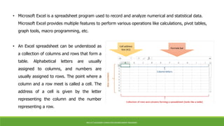
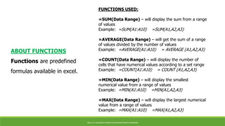
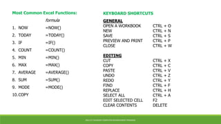
• Microsoft Excel is a spreadsheet program used to record and analyze numerical and statistical data.
Microsoft Excel provides multiple features to perform various operations like calculations, pivot tables,
graph tools, macro programming, etc.
• An Excel spreadsheet can be understood as
a collection of columns and rows that form a
table. Alphabetical letters are usually
assigned to columns, and numbers are
usually assigned to rows. The point where a
column and a row meet is called a cell. The
address of a cell is given by the letter
representing the column and the number
representing a row.

Running Excel is like running any
other Windows program. If you
are running Windows with a GUI
like (Windows XP, Vista, and 7)
follow the following steps.
1. Click on start menu
2. Point to all programs
3. Point to Microsoft Excel
4. Click on Microsoft Excel
For Windows 8. Follow the following steps
to run Excel on Windows 8.1
Click on Start Menu
Search for Excel even before you even start
typing, all programs starting with what you
have typed will be shown.
Click on Microsoft Excel
The following image shows you how to do
this
HOW TO OPEN MICROSOFT EXCEL?

MICROSOFT EXCEL ENVIRONMENT

UNDERSTANDING THE RIBBON
The ribbon provides shortcuts to commands in Excel. A command is an action that the user performs. An
example of a command is creating a new document, printing a documenting, etc. The image below shows
the ribbon used in Excel 2013.

RIBBON COMPONENTS EXPLAINED
 Ribbon start button – it is used to access
commands i.e., creating new documents, saving
existing work, printing, accessing the options for
customizing Excel, etc.
 Ribbon tabs – the tabs are used to group similar
commands together. The home tab is used for
basic commands such as formatting the data to
make it more presentable, sorting and finding
specific data within the spreadsheet.
 Ribbon bar – the bars are used to group similar
commands together. As an example, the
Alignment ribbon bar is used to group all the
commands that are used to align data together.

VOCABULARY
Microsoft Excel is a spreadsheet program. We use it to
create reports that need calculations and charts.
1. An Excel file is called a Workbook.
- Default title is Book1
2. Ribbon broken into Tabs (Home, Insert, Page Layout…)
- Tabs broken into groups (Clipboard, Font, Alignment)
3. Name box (left) and formula bar (right)
- Name box shows address of current cell
- Formula bar shows contents of current cell
4. Columns Headings are Lettered, Rows Headings are
Numbered
- Columns of a building, rows of chairs
5. Worksheet navigation buttons, Worksheet tabs
- Sheet1
6. Status bar
- Excel behaves differently depending on the current
"mode"

STATUS BAR MODES
1. Ready mode. This means
nothing is being entered or
edited on the spreadsheet.
2. Enter mode. This mode is
when you are doing data entry,
just typing in the contents.
3. Edit mode. Edit the contents
of the current cell. Double‐click
on a cell with data in it, or click
inside the formula bar for this
mode.
4. Point mode. Used when
linking to cell addresses within
a formula or from an Excel
dialog window.
KEYBOARD NAVIGATION

Fill Handle
The Fill Handle is in the bottom right corner of the selected cell. When you place your mouse over this handle, it
changes from a thick white cross to a thin black cross. Once you see the thin cross (no arrows) you can click and
drag the cell to fill its contents in a single direction (up, down, left, or right). If you want to go in two directions,
you must first complete one way, let go of the mouse and then drag the handle in the second direction.
When you use the Fill Handle to pull down a single number or plain text, it will copy the data. When you use the
Fill Handle to pull down a text with numbers, a date, a month, or a weekday it will fill in a series.

Formula
The Equal Sign
To start a formula one needs to type in the equal sign (=) first. The equal sign indicates that the current
cell in the worksheet holds a formula.
Parts Of A Formula
Operators
+ (addition) - (subtraction) * (multiplication) / (division) ^ (exponent/power)
These Are The Data That You Can Use As Operands
a) numbers (1, 3, 88.8, 23, etc.) Note: #### means that the cell is just not wide enough to
accommodate the numbers
b) cell names (A1, B6, C9, AB62, etc.)
c) another formula
d) a function
Examples Of A Formula:
= 100 + 8 = A1 – A2 = 8 + A2 = (A2 + 5) – (B2 * 9) =5/2
= 5^2 result 25

AutoSum
We can build equations to do math on many cells, but there are functions built into Excel
that can help us automate the most common ones: Sum, Average, Count, Maximum, Minimum. On the
far right of the Home tab you'll find the sigma (Σ).
When you click on the word AutoSum, you'll get a sum function. There is a dropdown list at the end of the
button that will show more function options. The AutoSum button looks for numbers above or to the left of
the cell to choose the range (the set) of numbers. Make sure to press enter or click the check to accept as
soon as the function shows up. If you click outside the cell while you see the function, you may break the
equation.

Freeze Panes (Lock Titles to Top of Page)
1) Press Ctrl‐Home on the keyboard to return to Cell A1
2) Turn to the View Tab in the Ribbon
3) Find the Option Freeze Panes
a. Choose Freeze Top Row
b. b. Scroll down through the worksheet to see the titles in Row 1 stay at the top

FUNCTIONS USED:
=SUM(Data Range) – will display the sum from a range
of values
Example: =SUM(A1:A10) =SUM(A1,A2,A3)
=AVERAGE(Data Range) – will get the sum of a range
of values divided by the number of values
Example: =AVERAGE(A1:A10) = AVERAGE (A1,A2,A3)
=COUNT(Data Range) – will display the number of
cells that have numerical values according to a set range
Example: =COUNT(A1:A10) = COUNT (A1,A2,A3)
=MIN(Data Range) – will display the smallest
numerical value from a range of values
Example: =MIN(A1:A10) =MIN(A1,A2,A3)
=MAX(Data Range) – will display the largest numerical
value from a range of values
Example: =MAX(A1:A10) =MAX(A1,A2,A3)
ABOUT FUNCTIONS
Functions are predefined
formulas available in excel.

IF FUNCTION
ABOUT THE IF FUNCTION
IF is a logical function that allows you to display a result if a certain condition is met.
PARTS OF THE IF FUNCTION
=IF(Logical Test, Value if True, Value if False)
The logical test contains the criteria/condition. The Value if True will be displayed when the criteria/condition is
satisfied. Otherwise, the Value if False is displayed.
CONDITIONAL OPERATORS USED IN LOGICAL TEST:
= Equals
> greater than
< less than
>= greater than or equal
<= less than or equal
EXAMPLE OF IF STATEMENTS:
=IF(A1>50, “GOOD”, “BAD”)

Most Common Excel Functions:
formula
1. NOW =NOW()
2. TODAY =TODAY()
3. IF =IF()
4. COUNT =COUNT()
5. MIN =MIN()
6. MAX =MAX()
7. AVERAGE =AVERAGE()
8. SUM =SUM()
9. MODE =MODE()
10.COPY
GENERAL
OPEN A WORKBOOK CTRL + O
NEW CTRL + N
SAVE CTRL + S
PREVIEW AND PRINT CTRL + P
CLOSE CTRL + W
EDITING
CUT CTRL + X
COPY CTRL + C
PASTE CTRL + V
UNDO CTRL + Z
REDO CTRL + Y
FIND CTRL + F
REPLACE CTRL + H
SELECT ALL CTRL + A
EDIT SELECTED CELL F2
CLEAR CONTENTS DELETE
KEYBOARD SHORTCUTS

1. Select the cell or column that contains the text you want to split.
2. Select Data > Text to Columns.
3. In the Convert Text to Columns Wizard, select Delimited > Next.
4. Select the Delimiters for your data. For example, Comma and Space. You can see a preview of your data in
the Data preview window.
5. Select Next.
6. Select the Destination in your worksheet which is where you want the split data to appear.
7. Select Finish.
SPLIT TEXT INTO DIFFERENT COLUMNS WITH THE
CONVERT TEXT TO COLUMNS WIZARD

ms-excel.pptx

More Related Content

What's hot

Similar to ms-excel.pptx

More from Moises Tenyosa

Recently uploaded

ms-excel.pptx