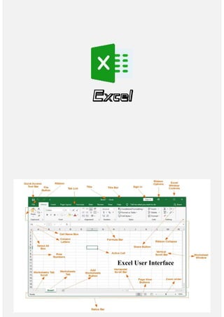
Microsoft Excel is a spreadsheet program used for recording and analyzing numerical data, consisting of rows and columns that form cells. It offers various tools for data manipulation, analysis, and visualization, including formulas and functions to summarize and compute large datasets. Key features include the ribbon interface for command shortcuts, templates for specific tasks, and extensive capabilities for graphing, conditional formatting, and data presentation.

1. Excel
Excel User Interface

2. Excel 01
What is Microsoft Excel?
Microsoft Excel is a spreadsheet program that is used to record and analyze
numerical data. A spreadsheet can be thought as a collection of columns and
rows that form a table.
Rows and Columns: Alphabetical letters (A,B,C ) are usually
assigned to columns and numbers (1,2,3 ) are usually assigned to rows.
Cell: The point where a column and a row meet is called a cell. The
address of a cell is given by the letter representing the column and the
number representing a row. E.g.: A20, E12, D2 etc.
Cell Range: A group of cells is known as a cell range. Rather than a
single cell address, you will refer to a cell range using the cell addresses
of the first and last cells in the cell range, separated by a colon. For
example, a cell range that included cells A1, A2, A3, A4, and A5 would
be written as A1:A5.
Why learn Microsoft Excel?
We all deal with numbers in one way or the other. We all have daily
expenses which we pay for from the monthly income that we earn. For
one to spend wisely, they will need to know their income vs.
expenditure. Microsoft Excel comes in handy when we want to record,
analyze and store such numeric data.
One of the best uses of MS Excel is that you can analyze larger amounts of
data to discover trends. With the help of graphs and charts, you can
summarize the data and store it in an organized way so that whenever you
want to see that data then you can easily see it.
There are wonderful tools for sorting, filtering and searching which all the
more make you work easy.
It makes easy for you to solve complex mathematical problems in a much
simpler way without much manual effort. There are so many formulas in
MS Excel and by using these formulas you can implement lots of
operations like finding sum, average, etc. on a large amount of data all at
once.
The chief use of MS Excel is that it provides security for excel files so
people can keep their files safe. All the files of MS Excel can be kept
password-protected through visual basic programming or directly within
the excel file.
It helps you in adding more sophistication to your data presentations
which means that you can improve the data bars, you can highlight any
specific items that you want to highlight and make your data much more
presentable easily.
You can represent data in the form of charts and graphs so it can help in
identifying different trends. With the help of MS Excel, trend lines can be
extended beyond graph and therefore, it helps one in analyzing the trends
and patterns much easier. In business, it is very important to analyze the
popularity of goods or the selling pattern that they follow to maximize
sales.
MS Excel helps in managing expenses.
Worksheet is a collection of rows and columns. When a row and a
column meet, they form a cell. Cells are used to record data. Each cell is
uniquely identified using a cell address. Columns are usually labelled
with letters while rows are usually numbers.
Workbook is a collection of worksheets. By default, a workbook has
three cells in Excel. You can delete or add more sheets to suit your
requirements. By default, the sheets are named Sheet1, Sheet2 and so on
and so forth. You can rename the sheet names to more meaningful
names i.e. Daily Expenses, Monthly Budget, etc.
Understanding the Ribbon
The ribbon provides shortcuts to commands in Excel. A command is an
action that the user performs. An example of a command is creating a new
document, printing a documenting, etc.
Ribbon start button - it is used to access commands i.e. creating new
documents, saving existing work, printing, accessing the options for
customizing Excel, etc.
Ribbon tabs the tabs are used to group similar commands together. The
home tab is used for basic commands such as formatting the data to make
it more presentable, sorting and finding specific data within the
spreadsheet.
Ribbon bar the bars are used to group similar commands together. As
an example, the Alignment ribbon bar is used to group all the commands
that are used to align data together.
Template: A template is a preformatted workbook designed for a specific purpose
such as tracking sales or budgeting.
Merge cells A highly useful feature used by accountants is the merge facility
which enables two or more neighboring cells to be merged into a single larger cell.
There are a number of options, the two most common being:
Merge and center Merges all selected cells into a single cell retaining only the
contents of the upper-left most cell. The result is center/bottom aligned.
Merge across Merges selected cells on a line by line basis, again retaining only
the contents of the left-most cells. The result is left aligned.
Freeze panes (lock rows / columns) Freezing panes or splitting panes enables
you to keep an area of a worksheet visible whilst you scroll to another area of the
worksheet. The difference between freezing and splitting is that with freezing you
continue to view just one view of the worksheet, whereas with splitting panes the
screen effectively becomes either two or four views of the underlying worksheet.
Cloud computing: Cloud computing is the use of computing resources (both
software and hardware) that are delivered as a service over a network typically
the internet. A recent trend has been for users to store files off-site rather than
within their own computer and access their files via the internet. This has the
benefit of users being able to access their files from any location (subject to an
internet connection).
Freeze panes: Reviewing a worksheet by holding the same columns &
sliding others
SHIFT + F3 displays the function insert dialog window
SHIFT + F11 Creates (chart) a new worksheet
F2 Check formula and cell range covered
Alt + Enter to insert a new line in the same cell
Ctrl + 0 to hide entire column
Ctrl + ;/ =TODAY() to insert current date in a cell
=NOW() to insert current date and time
=COUNTA() counts non-empty cells
$ symbol specifies the fixed columns o rows
We will now perform the calculations using the respective arithmetic operators.
When performing calculations in Excel, you should always start with the equal (=)
sign.
FORMULA IN EXCEL: is an expression that operates on values in a range of
cell addresses and operators. For example, =A1+A2+A3, which finds the sum of
the range of values from cell A1 to cell A3. An example of a formula made up of
discrete values like =6*3. =A2 * D2 / 2
Mistakes to avoid: Remember the rules of Brackets of Division, Multiplication,
Addition, & Subtraction (BODMAS). This means expressions are brackets are
evaluated first. For arithmetic operators, the division is evaluated first followed by
multiplication then addition and subtraction is the last one to be evaluated. Using
this rule, we can rewrite the above formula as =(A2 * D2) / 2. This will ensure that
A2 and D2 are first evaluated then divided by two.
Excel spreadsheet formulas usually work with numeric data; you can take
advantage of data validation to specify the type of data that should be accepted by
a cell i.e. numbers only.
To ensure that you are working with the correct cell addresses referenced in the
formulas, you can press F2 on the keyboard. This will highlight the cell addresses
used in the formula, and you can cross check to ensure they are the desired cell
addresses.
When you are working with many rows, you can use serial numbers for all the
rows and have a record count at the bottom of the sheet. You should compare the
serial number count with the record total to ensure that your formulas included all
the rows.
FUNCTION IN EXCEL: is a predefined formula that is used for specific
values in a particular order. Function is used for quick tasks like finding the sum,
count, average, maximum value, and minimum values for a range of cells. For
example, cell A3 below contains the SUM function which calculates the sum of
the range A1:A2.
SUM for summation of a range of numbers
AVERAGE for calculating the average of a given range of numbers
COUNT for counting the number of items in a given range
Importance Of Functions: Functions increase user productivity when working with
excel. Let's say you would like to get the grand total for the above home supplies
budget. To make it simpler, you can use a formula to get the grand total. Using a
formula, you would have to reference the cells E4 through to E8 one by one. You
would have to use the following formula.
= E4 + E5 + E6 + E7 + E8
With a function, you would write the above formula as
=SUM (E4:E8)
As you can see it is much more efficient to use a function to get the sum than
using the formula which will have to reference a lot of cells.

3. Excel 02
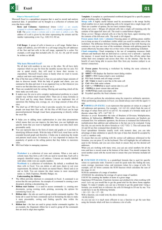
Symbol Name Description
= Equal to Every Excel Formula must begins with Equal to symbol (=).
Example:=A1+A5
() Parentheses All Arguments of the Excel Functions specified between the Parentheses.
Example:=COUNTIF(A1:A5,5)
() Parentheses Expressions specified in the Parentheses will be evaluated first. Parentheses changes
the order of the evaluation in Excel Formula.
Example: =25+(35*2)+5
* Asterisk Wild card operator to denote all values in a List. (Multify)
Example:
, Comma List of the Arguments of a Function Separated by Comma in Excel Formula.
Example:
& Ampersand Concatenate Operator to connect two strings into one in Excel Formula.
Example:
$ Dollar Makes Cell Reference as Absolute in Excel Formula. (Freeze the range)
Example:=SUM($B$2:$B$25)
! Exclamation Sheet Names and Table Names Followed by ! Symbol in Excel Formula.
Example: =SUM(Sheet2!B2:B25)
[]
Square
Brackets Uses to refer the Field Name of the Table (List Object) in Excel Formula.
Example:=SUM(Table1[Column1])
{}
Curly
Brackets Denote the Array formula in Excel.
Example: {=MAX(A1:A5-G1:G5)}
: Colon Creates references to all cells between two references (Create a range).
Example: =SUM(B2:B25)
, Comma Union Operator will combine the multiple references into One.
Example: =SUM(A2:A25, B2:B25)
(space) Space Intersection Operator will create common reference of two references.
Example: =SUM(A2:A10 A5:A25)
"" Blank Blank
" " Space When we use space.
?
Question
marks When we wnt to represent as a single character.
~ Tilde When we represent single chracter in formula.
# Hash When we represent numeric.
* Astrisk/Star When we represent to text.
@
At/ At the
rate Represent text in custom format.
^ Carret It's a symbol of cube.
> Greater than
< Less than
>= Greater than or equal
<= Less than or equal
<> Not equal
+ Plus/Sum Add all the values in a cell range.
-
Minus/Hyph
en Deduct the value from a cell range.
/
Divided/Slas
h Divide the value of a cell or cell range.
Important symbol in excel:
Ctrl + A = Select all
Ctrl + B = Bold
Ctrl + C = Copy
Ctrl + D = Fill down
Ctrl + E = Flash
Ctrl + F = Find
Ctrl + G = Go to
Ctrl + H = Replace
Ctrl + I = Italic
Ctrl + J = (Nothing)
Ctrl + K = Hyperlink
Ctrl + L = Insert table
Ctrl + M = (Nothing)
Ctrl + N = Create New workbook
Ctrl + O = Open workbook
Ctrl + P = Print
Ctrl + Q = (Nothing)
Ctrl + R = Fill right
Ctrl + S = Save
Ctrl + T = Insert table
Ctrl + U = underline
Ctrl + V = paste
Ctrl + W = Closing Workbook
Ctrl + X = Cut
Ctrl + Y = Redo
Ctrl + Z = Undo
F1 Help
F2 Edit Mode
F3 Paste Name Formula
F4 Repeat Action
F5 Go To
F6 Next Pane
F7 Spell Check
F8 Extended Selection
F9 Calculate All
F10 Activate Menu
F11 New Chart
F12 Save As

4. Excel 03
FUNCTION DESCRIPTION USAGE
SUM
Adds all the values in a
range of cells
=SUM(E4:E8)
MIN
Finds the minimum
value in a range of cells
=MIN(E4:E8)
MAX
Finds the maximum
value in a range of cells
=MAX(E4:E8)
AVERAGE
Calculates the average
value in a range of cells
=AVERAGE(E4:E8)
COUNT
Counts the number of
cells in a range of cells
=COUNT(E4:E8)
COUNTA
The COUNTA
function counts cells
that contain values,
including numbers,
text, logical, errors, and
empty text ("").
=COUNTA(A1:A10)
COUNTIF
To count the number of
cells that meet a
criterion;
=COUNTIF(B2:B5,">55")
LEN
Returns the number of
characters in a string
text
=LEN(B7)
SUMIF
Adds all the values in a
range of cells that meet
a specified criteria.
=SUMIF(range,criteria,
[sum_range])
AVERAGEIF
Calculates the average
value in a range of cells
that meet the specified
criteria.
=AVERAGEIF(range,c
riteria,[average_range])
8)
DAYS
Returns the number of
days between two dates
=DAYS(D4,C4)
NOW
Returns the current
system date and time
=NOW()
MEDIAN To calculate median =MEDIAN(C2:C8)
MODE To calculate mode =MODE(C2:C8)
CONCAT
CONCAT function
combines the text from
multiple ranges and/or
strings
=CONCAT(B2," ", C2)
SEPARTE
Common Function
FUNCTION DESCRIPTION USAGE
ISNUMBER
Returns True if the
supplied value is
numeric and False if it
is not numeric
=ISNUMBER(A3)
RAND
Generates a random
number between 0
and 1
=RAND()
ROUND
Rounds off a decimal
value to the specified
number of decimal
points
=ROUND(3.14455,2)
MEDIAN
Returns the number in
the middle of the set
of given numbers
=MEDIAN(3,4,5,2,5)
PI
Returns the value of
=PI()
POWER
Returns the result of a
number raised to a
power.
POWER( number,
power )
=POWER(2,4)
MOD
Returns the
Remainder when you
divide two numbers
=MOD(10,3)
ROMAN
Converts a number to
roman numerals
=ROMAN(1984)
Numeric Functions:
FUNC. DESCRIPTION USAGE COMMENT
LEFT
Returns a number of
specified characters from
the start (left-hand side)
of a string
Left 4
Characters of
RIGHT
Returns a number of
specified characters from
the end (right-hand side)
of a string
2)
Right 2
Characters of
MID
Retrieves a number of
characters from the
middle of a string from a
specified start position
and length.
=MID (text, start_num,
num_chars)
Retrieving
Characters 2
to 5
ISTEXT
Returns True if the
supplied parameter is
Text
=ISTEXT(v
alue)
value The
value to
check.
FIND
Returns the starting
position of a text string
within another text
string. This function is
case-sensitive.
=FIND(find_text,
within_text,
[start_num])
,1)
Find oo in
Result is 2
REPLA
CE
Replaces part of a string
with another specified
string.
=REPLACE (old_text,
start_num, num_chars,
new_text)
=REPLAC
oo
String functions:
FUNCTION DESCRIPTION USAGE
DATE
Returns the number that
represents the date in excel code
=DATE(2015,2,4)
DAYS
Find the number of days between
two dates
=DAYS(D6,C6)
MONTH
Returns the month from a date
value
MINUTE
Returns the minutes from a time
value
YEAR
Returns the year from a date
value
Date Time Functions:

5. Excel 04
Logical Functions: are used in spreadsheets to test whether a situation is true or false. Depending on the result of
that test, you can then elect to do one thing or another. These decisions can be used to display information, perform
different calculations, or to perform further tests. Such as: =IF(Condition,x,y)
The IF Function
The IF function is the key logical function used for decision making. It takes the format:
=IF(condition, true, false)
For example, you could use the following formula:
=IF(B2 > 400, where,
B2 > 400 is the condition being tested
(this could be translated as the value in cell B2 greater than 400
is the text to display if B2 is greater than 400 (the result of the test is yes or TRUE)
is the text to display if B2 is less than or equal to 400 (the result of the test is no or FALSE)
The AND Function
The AND function is used to compare more than one condition. It returns TRUE only if all of the conditions are
met, and takes the format:
=AND(condition1, condition2, )
For example, you could use the following formula:
=AND(B2 > 400, C2 < 300) where,
B2 > 400 is the first condition being tested
C2 < 300 is the second condition being tested
This will only return the result TRUE if the value in cell B2 is greater than 400 and the value in cell C2 is less
than 300. In all other situations, the result will be FALSE.
The OR Function
The OR function is also used to compare more than one condition. It returns TRUE if any of the conditions are
met, and takes the format:
=OR(condition1, condition2, )
For example, you could use the following formula:
=OR(B2 > 400, C2 < 300) where,
B2 > 400 is the first condition being tested
C2 < 300 is the second condition being tested
This will return the result TRUE if either the value in cell B2 is greater than 400 or the value in cell C2 is less
than 300. The result will be FALSE only if neither of the conditions is met.
Example:
=IF(A1>33
=IF(A1<20000,E5*10%,E5*20%)
Suppose, the value of cell A1 in MS Excel sheet is 3500. If we
apply the formula =IF(A1<20000,A1*10%,A1*20%) what
will be the result?
Suppose cells A1 and B1 contain the values 30000 and 100,
respectively. If we apply the formula
=IF(A1<>20000,B1*10%,B1*20%), what will be the result in
C1?

6. Excel 05
VLOOKUP function
The VLOOKUP function is used to perform a vertical look up in
the left most column and return a value in the same row from a
column that you specify. explain this in a language.
The home supplies budget has a serial number column that
uniquely identifies each item in the budget. Suppose you have the
item serial number, and you would like to know the item
description, you can use the VLOOKUP function. Here is how the
VLOOKUP function would work.
=VLOOKUP (C12, A4:B8, 2, FALSE)
HERE,
"=VLOOKUP" calls the vertical lookup function
"C12" specifies the value to be looked up in the left most column
"A4:B8" specifies the table array with the data
"2" specifies the column number with the row value to be returned
by the VLOOKUP function
"FALSE," tells the VLOOKUP function that we are looking for an
exact match of the supplied look up value
Data Filters
Use AutoFilter or built-in comparison operators like "greater than" and 10 in Excel to show the data you want and hide the rest. Once you
filter data in a range of cells or table, you can either reapply a filter to get up-to-date results, or clear a filter to redisplay all of the data.
Data filters allow us to get data that matches our desired criteria.
Let's say we want to show the results of all the students whose names start with "ja" or get scores that are less than, greater than or equal to
a certain value, we can use filters to get such data.
Select the name and scores columns as shown below-
Click on the Name Filter
Select text filters
Select begins with
You will get the following window.
Enter "ja" and click on "OK" button
You should be able to see only the results for Jane and James.

7. Excel 06
Data validation
Data validation is very important in the sense that it helps us
avoid mistakes that can be avoided. assume you are
recording student exam marks and you know the minimum is 0
and the maximum is 100. You can take advantage of validation
features to ensure that only values between 0 and 100 are entered.
Add a new sheet in your workbook by clicking on the plus button
at the bottom of the worksheet.
Add a column for S/N, Name and Score. Your sheet should look as
follows:
S/N Name Score
1 Jane
2 James
3 Jones
4 Jonathan
5 John
Click on the DATA tab
Select the cells C2 to C6 (The cells that will be used to
record the scores)
Click on Data validation drop down list.
Click on Data validation.
Click on Error Alert tab
Enter the alert title and message as shown in the
diagram below.
Click on OK button
Try to enter a score greater than 100. You will get
the following error message
You will get the following dialogue window

8. Excel 07
Group and Ungroup
Groups allow to view easily and hide unnecessary details from either columns or rows. In addition to that, we
can also use groups to analyze data that belongs to a common category.
Let's illustrate this with an example. We will use the student scores example above.
Right click on the score and select insert
column. Name the name column gender.
Change James to Juanita. Put female for Janet
and Juanita. Put male for the rest of the
students. You sheet should look as follows.
We will now group the females together and
display their average score and do the same for
the males.
Click on DATA tab on the ribbon
Select all the columns and rows with data
Click on Group drop down button as shown
in the image below
You will get the following window- and click
on OK
We will now calculate the average scores for
females and males
Select the whole data as shown below
Click on Subtotal drop down button under DATA
tab
You will get the following window-
Set "At each change" into gender
Set "Use function" to average
Select "Add subtotal" to Score
Click on "OK" button