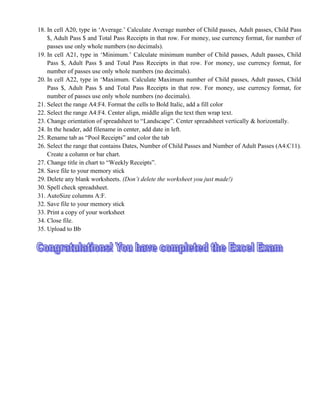
1) The manager of King Neptune's Community Pool needs a worksheet analyzing weekly receipts of child and adult pool passes.
2) The worksheet should include data on the number of child and adult passes sold each day from June 1-7, calculate receipts for each day and totals, and include averages, minimums, and maximums.
3) Additional formatting and calculations are required, such as merging and formatting text, adding borders and colors, creating formulas to calculate daily and total receipts, and inserting a chart to visualize the weekly receipts data.
Excel – is the world’s most widely used spreadsheet calculating program
It is used in many places like hospitals, hotels, school and companies etc.
A program that allows you to use data to forecast, manage, predict, and present information
Lets Just Go For It! Wish you an Awesome Leaning Experience.
Subscribe to our YouTube channel: https://www.youtube.com/c/TimesRide?sub_confirmation=1
Our Official Website: http://timesride.com
Follow us:
Facebook: https://www.facebook.com/rs.agrawal.9026
Instagram: https://www.instagram.com/timesridenetwork/
Twitter: https://twitter.com/TimesRide
Pinterest: https://in.pinterest.com/ride0472/
Thank You
#AwesomeLearningExperience
#SmartQuickTips&Tricks #LeaningVideos #TimesRide #Keep Learning to Keep Winning!
MS Excel Learning for PPC Google AdWords Training CourseRanjan Jena
MS Excel learning to get expertise in Google AdWords training course. Learn all important tips and techniques in MS Excel for your fast and easy approach to Google AdWords analysis and reporting formats.
Ranjan Jena conducts Adwords Training session in Bangalore, currently with more than 45 students already graduated under his guidance and mentorship. For any training need, you can directly reach him at +91-7760969452
Handout used by the Westerville Public Library for the Introduction to Excel 2007 class. Provides basic information about creating a spreadsheet using Microsoft Excel 2007.
Excel Practical - Exercise 4 Insert the following tabBetseyCalderon89
Excel Practical - Exercise 4
Insert the following table into Sheet1 of an Excel spreadsheet, keeping the
cell references consistent.
1. Copy the data from the table (3rd page) into an new Excel Spreadsheet.
Keep the data as indicated on the columns and rows.
2. Save your work as: yourname_P4
3. Add the column title (D1): Humor Rating (out of 10)
CALCULATIONS
4. Calculate the Humor Rating based on the scores on the 2nd set of
numbers (table starts in cell A10)
a. Format these numbers to only 1 decimal point
CHARTING
5. Create a 3-D Column Chart. Chart the Humor Rating and Muppet Name
a. Place the chart in a new worksheet title: Humor Rating
b. Color the tab Blue
c. Show the Muppets Names and Humor Rating on the chart
a. Use data labels
FORMATTING
6. Insert 2 rows at the top of the worksheet
7. Add the title (A1): The Muppets - Vital Statistics
a. Center the title across the table
b. Make it bold and underline it
c. Chose the color and size font that is appropriate
8. Color each row with the color indicated in column C for each muppet.
9. Format the rest of the table to your liking.
a. Choose appropriate fonts
b. Choose appropriate border
10. Format the Humor Rating table to your liking
a. Place borders around all of the cells
b. Center the Scores
11. Bold the Column title in Row 3 and center them
12. Change the Tab Name and color to: Muppets and color it purple
13. Use Conditional Formatting to color the Humor Rating of 7.3 and
higher to Bold White Font with a Dark Blue Background
14. Fix the column widths so that you can see all of the data
15. Change the worksheets to Landscape orientation
FINISHING TOUCHES
16. Insert a header in the center section.
a. Type your name and <enter>
b. Type the course ID (CGS1030)
17. Insert an image of the Muppets to the right of the table
18. Change the Document Properties
a. Include your name
b. Subject
c. Tags (minimum of 3 – separate by commas)
A B C D E F G H I J K
1 Muppet Name Creature
Type
Color
2 Kermit Frog Green
3 Miss Piggy Swine Pink
4 Waldorf &
Statler
Grumpy Men Pink
5 Gonzo Unknown Blue/Gray
6 Animal Percussionist Red
7 Swedish Chef Swede Tan
8 Fozzie Bear Brown
9
10 Humor Rating
11 Score 1 Score 2 Score 3 Score 4 Score 5 Score 6 Score 7 Score 8 Score 9 Score 10
12 Kermit 6 5.8 6.3 8.122 8.3 7.55 7.6 8.5 7.1 6.6
13 Miss Piggy 4.3 5.6 3.8 7.53 8.4 6.8 4.9 8.1 9.1 7.7
14 Waldorf &
Statler
4.9 4.9 9.2 8.4 7.5 9.64 8.3 4.5 9.64 9.62
15 Gonzo 8.2 5.7 5.79 7.5 8 7.2 9.4 5.9 8.32 8.4
16 Animal 7.6 3.9 6.8 9.26 4.68 7.9 7.2 6.1 6.9 5.66
17 Swedish Chef 7.6 4.8 4.82 4.9 6.8 8.22 6.8 7.9 7.28 8.3
18 Fozzie 6.7 8.9 3.2 8.3 8.34 7.5 9.12 8.45 7.88 8.12
Week 6 Assignment Template
In the land of free trade, the public does not view all ...
For more course tutorials visit
www.newtonhelp.com
BIS 155 Course Project Excel Project
BIS 155 Lab 1 of 7: Saddle River Marching Band
BIS 155 iLab 1 Upper Saddle River Marching Band (New)
BIS 155 Inspiring Innovation -- bis155.comkopiko101
For more course tutorials visit
www.bis155.com
BIS 155 Course Project Excel Project
BIS 155 Lab 1 of 7: Saddle River Marching Band
BIS 155 iLab 1 Upper Saddle River Marching Band (New)
BIS 155 Lessons in Excellence / bis155.comkopiko33
For more course tutorials visit
www.bis155.com
BIS 155 Course Project Excel Project
BIS 155 Lab 1 of 7: Saddle River Marching Band
BIS 155 iLab 1 Upper Saddle River Marching Band (New)
BIS 155 Lab 2 of 7: Excel's Advanced Formulas & Functions
Computer Applications Microsoft Excel2016 Graded Project.docxmccormicknadine86
Computer Applications : Microsoft Excel
2016 Graded Project
Lesson 4 Overview
In this lesson, you'll create a spreadsheet that tracks the cost of
elementary school supplies distributed to teachers over a two-month
period in order to illustrate correct usage of Microsoft Excel 2016.
4.1 Design a spreadsheet that tracks the cost of
elementary school supplies distributed to teachers over
a two-month period
Excel 2016
READING ASSIGNMENT
Your project must be submitted as an Excel workbook (.xlsx, .xls). Your
project will be individually graded by your instructor and therefore may take up
to five to seven days to grade. Be sure that each of your files contains the
following information:
Your name
Your student ID number
The exam number
Your email address
Note: If you have more than 10 attachments, you’ll need to collect all of your
files into a compressed folder. To do this, follow these instructions based on
Page 1Copyright Penn Foster, Inc. 2019
Course Version: 1
your operating system:
Windows: Select the files you want to compress, right-click and select
Send to. . . and then Compressed (zipped) folder
Mac: Select the files you want to compress, control-click and select
Compress
To submit your graded project, follow these steps:
Log in to your student portal.
Click on Take Exam next to the lesson you’re working on.
Find the exam number for your project at the top of the Project Upload
page.
Follow the instructions provided to complete your exam.
Be sure to keep a backup copy of any files you submit to the school!
Introduction
This project requires you to develop a spreadsheet that tracks the cost
of elementary school supplies distributed to teachers over a two-
month period. You’ll assume the role of Office Manager, who has
multiple responsibilities, including distributing and maintaining
classroom supplies. For this project, you must prepare an Excel
spreadsheet and chart that will be sent to the school District Manager.
Instructions
Create a Spreadsheet
1. Start Excel and create a new workbook.
2. Enter data as shown in Figure below, sizing columns as
necessary, and then save your file, naming it School Supplies.
Page 2Copyright Penn Foster, Inc. 2019
Course Version: 1
An image of a new excel workbook with data entered and named
School Supplies.
3. Merge and center cells A1 through H1. Format the school name
as Title style.
4. Merge and center cells A2 through H2. Format the label as
Heading 1 style.
5. Bold the labels in row 4 and right align the labels above numeric
values.
6. Format the Cost/Unit values as Currency with 2 decimal places.
Your spreadsheet should look like Figure below.
An image of the School Supplies excel workbook with formatted data.
Page 3Copyright Penn Foster, Inc. 2019
Course Version: 1
7. In column D, enter appropriate formulas to calculate the
September costs for each school supply. Your formulas must use
cell references. Format the calculated values as Currency wit ...
1. EXCEL PRACTICAL
You have been hired as a consultant for King Neptune’s Community Pool. The manager of King Neptune’s
Community Pool needs you to prepare a worksheet to help analyze weekly receipts of child pool passes and
adult pool passes. Perform the following steps on the spreadsheet:
1. Create the spreadsheet using the following data: Begin in cell A4. Re-format dates to mm/dd if
needed.
A
1
2
3
4
5
6
7
8
9
10
Dates
6/1
6/2
B
C
D
E
F
Number of
Child Passes
200
135
141
110
123
102
Number of
Adult Passes
95
72
70
55
61
95
Child Pass $
Totals
Adult Pass $
Totals
Total Pass
Receipts
2. Save workbook as: ExcelExam_Firstname_Lastname to your memory stick. Save periodically
during exam to be safe!
3. Format the A column to show the date as 6/1, 6/2, etc. AutoFill the dates beginning with 6/1 and 6/2.
Your final year should be 6/6. Center dates.
4. Add the following data to row 11:
6/7
189
99
5. In cell A1 type in “King Neptune‟s Community Pool”. Merge and center vertically and horizontally
over cells A1:F1. Use “Cambria” font. Change font size to 16. Bold and Italicize text.
6. In cell A2, type in “Pool Pass Receipts for the Week of June 1 – June 7”. Merge and center over
cells A2:F2. Use “Cambria” font. Change fort size to 14. Bold Text.
7. Add a fill color to cell A1
8. In cell A12, insert the word, „Totals‟. Bold and right-align.
9. Total each column in row 12
10. In cell A15, type in the words “Child Pass Price”.
11. In cell A16, type in the words “Adult Pass Price”.
12. In cell D15, type in $1.50. In cell D16, type in $3.00. Make both currency format.
13. Create a formula using an absolute cell reference to calculate Child Pass Receipts for each day. Put
that formula (and $ total) in cell D5:D11. The total should calculate in D12.
14. Create a formula using an absolute cell reference to calculate Adult Pass Receipts for each day. Put
that formula (and $ total) in cell E5:E11. The total should calculate in E12.
15. Calculate total passes receipts ($ earned each day) in F5:F11, with a grand total in F12.
16. Use Currency Format for the D5:F12, center align
17. Select the range B12:F12 and add a „Top and Double Bottom Border.‟
2. 18. In cell A20, type in „Average.‟ Calculate Average number of Child passes, Adult passes, Child Pass
$, Adult Pass $ and Total Pass Receipts in that row. For money, use currency format, for number of
passes use only whole numbers (no decimals).
19. In cell A21, type in „Minimum.‟ Calculate minimum number of Child passes, Adult passes, Child
Pass $, Adult Pass $ and Total Pass Receipts in that row. For money, use currency format, for
number of passes use only whole numbers (no decimals).
20. In cell A22, type in „Maximum. Calculate Maximum number of Child passes, Adult passes, Child
Pass $, Adult Pass $ and Total Pass Receipts in that row. For money, use currency format, for
number of passes use only whole numbers (no decimals).
21. Select the range A4:F4. Format the cells to Bold Italic, add a fill color
22. Select the range A4:F4. Center align, middle align the text then wrap text.
23. Change orientation of spreadsheet to “Landscape”. Center spreadsheet vertically & horizontally.
24. In the header, add filename in center, add date in left.
25. Rename tab as “Pool Receipts” and color the tab
26. Select the range that contains Dates, Number of Child Passes and Number of Adult Passes (A4:C11).
Create a column or bar chart.
27. Change title in chart to “Weekly Receipts”.
28. Save file to your memory stick
29. Delete any blank worksheets. (Don’t delete the worksheet you just made!)
30. Spell check spreadsheet.
31. AutoSize columns A:F.
32. Save file to your memory stick
33. Print a copy of your worksheet
34. Close file.
35. Upload to Bb
3. GRADING RUBRIC – EXCEL EXAM
NAME:
Skill
Value
Entered data correctly, accurately, in correct cells
5
Save workbook as: ExcelExam_Firstname_Lastname
1
Format and autofill dates
1
A1 type in “King Neptune‟s Community Pool”. Merge and center over cells A1:F1. Use
3
“Cambria” font. Change font size to 16. Bold and Italicize text
A2, type in “Pool Pass Receipts for the Week of June 1 – June 7”. Merge and center over
3
cells A2:F2. Use “Cambria” font. Change fort size to 14. Bold Text
Add fill color to cell A1
2
In A12, insert the word, „Totals‟. Bold and right-align
2
Totals formulas correct in row 12
3
In cell D15, type in $1.50. In cell D16, type in $3.00. Make money currency format
1
Create a formula using an absolute value to calculate Child Pass Receipts for each day. Put
5
that formula (and $ total) in cell D5:D11
Create a formula using an absolute value to calculate Adult Pass Receipts for each day. Put
5
that formula (and $ total) in cell E5:E11
Calculate total passes receipts in F5:F12
5
Use Currency Format for the D5:F12
1
Select the range B12:F12 and add a „Top and Double Bottom Border.‟
1
In cell A20, type in „Average.‟ Calculate Average number of Child passes, Adult passes,
Child Pass $, Adult Pass $ and Total Pass Receipts. Correct formatting
3
In A21, type in „Minimum.‟ Calculate minimum number of Child passes, Adult passes,
Child Pass $, Adult Pass $ and Total Pass Receipts. Correct formatting
In A22, type in „Maximum‟. Calculate Maximum number of Child passes, Adult passes,
Child Pass $, Adult Pass $ and Total Pass Receipts. Correct formatting
3
3
Select the range A4:F4. Format the cells to Bold Italic, add fill color, center align, middle
align the text then wrap text
3
Change to “Landscape”. Center spreadsheet vertically/horizontally
1
Header: filename in center, date in left
1
Rename tab as “Pool Receipts”. Color tab
2
Select the range that contains Dates, # of Child Passes and # of Adult Passes (A4:C11).
Create a column or bar chart.
10
Change title in chart to “Weekly Receipts”
3
Autofit & print worksheet
2
Delete any blank worksheets, Save, close & upload file
1
Total
70
Earned