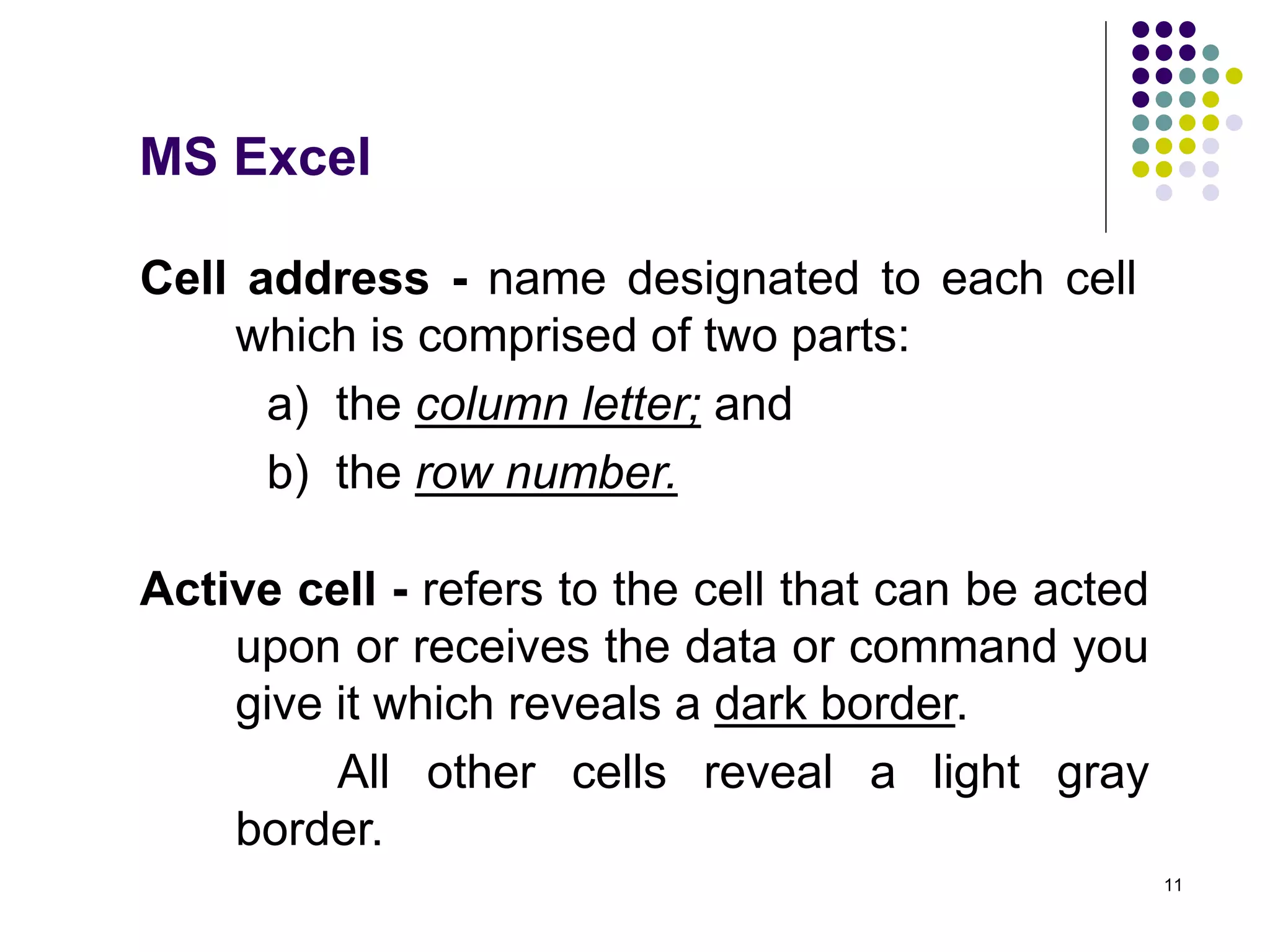
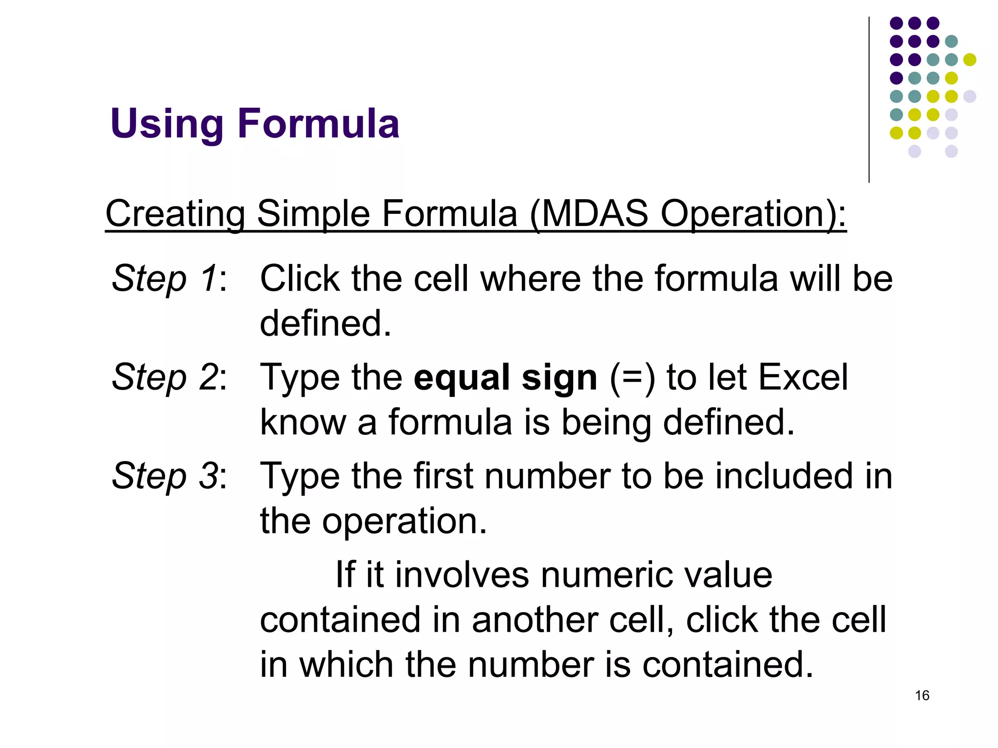
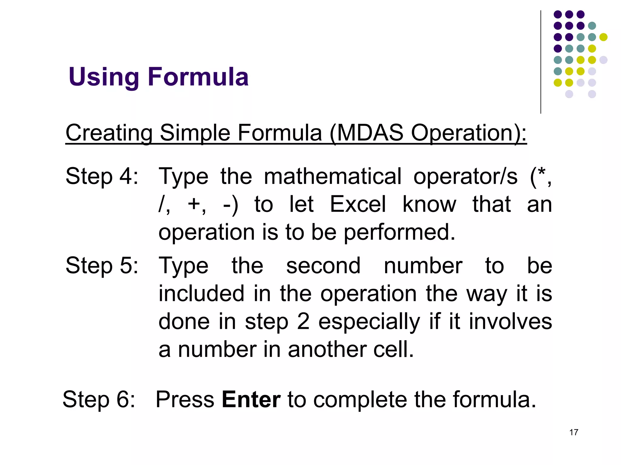
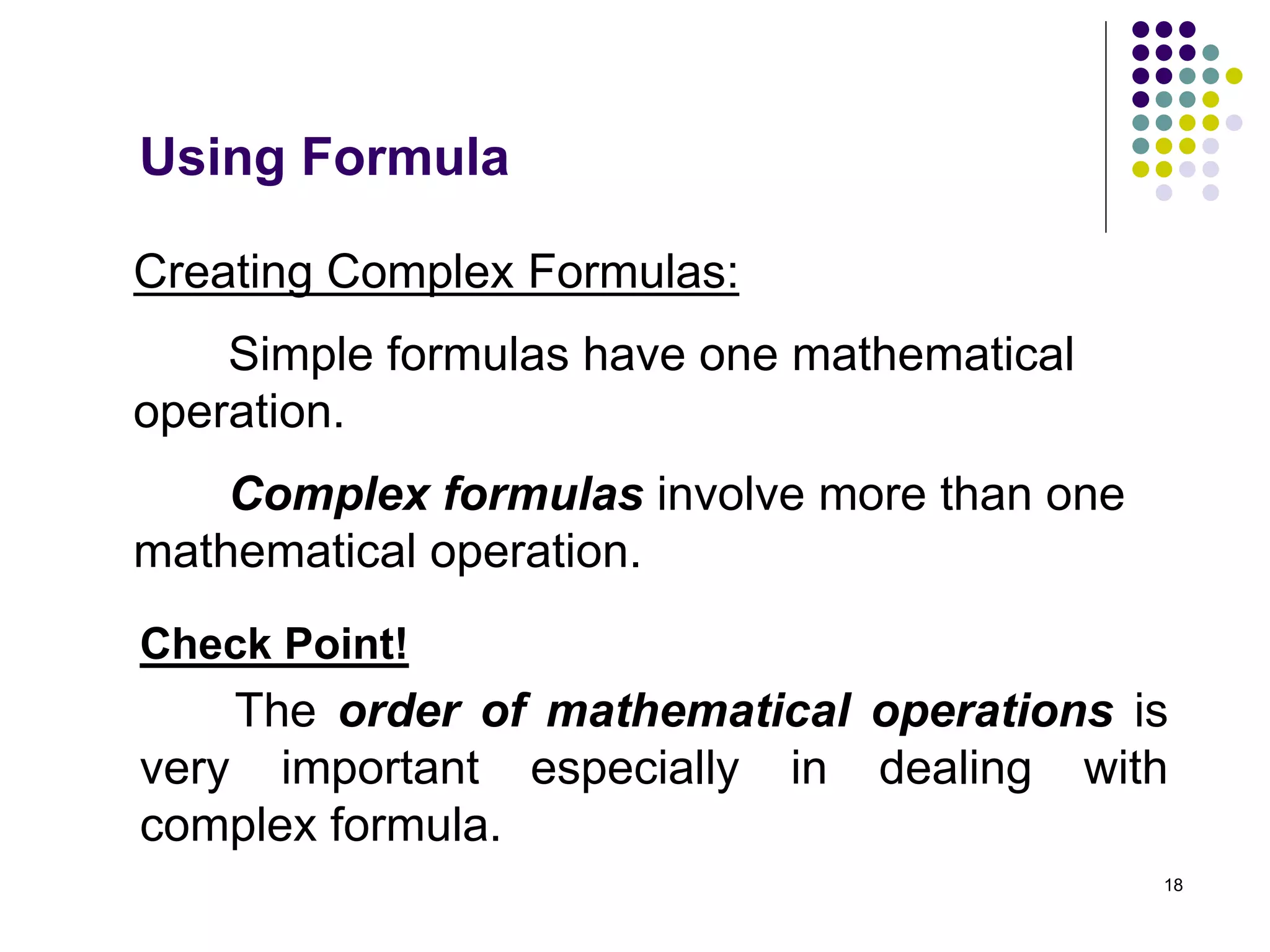
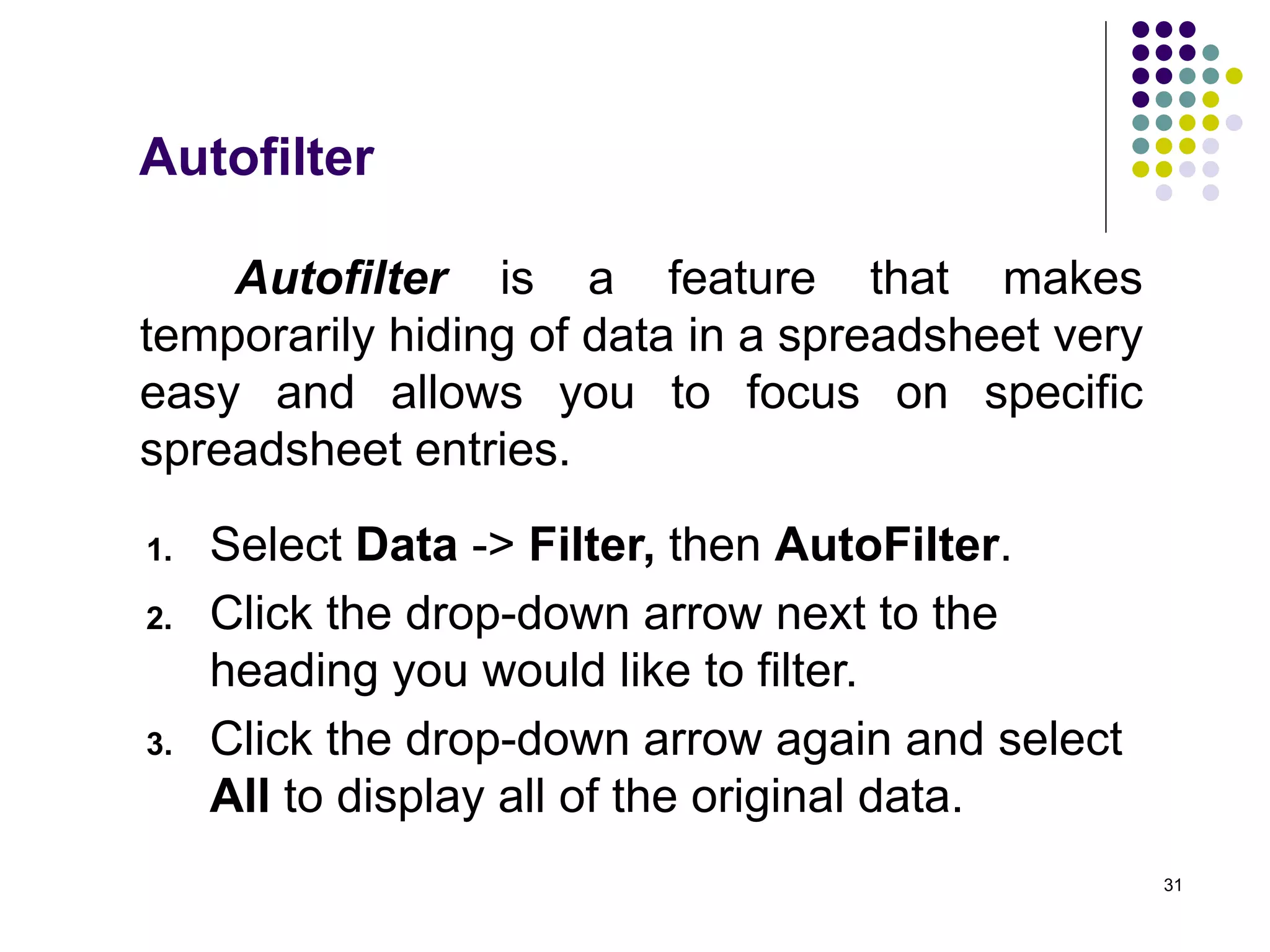
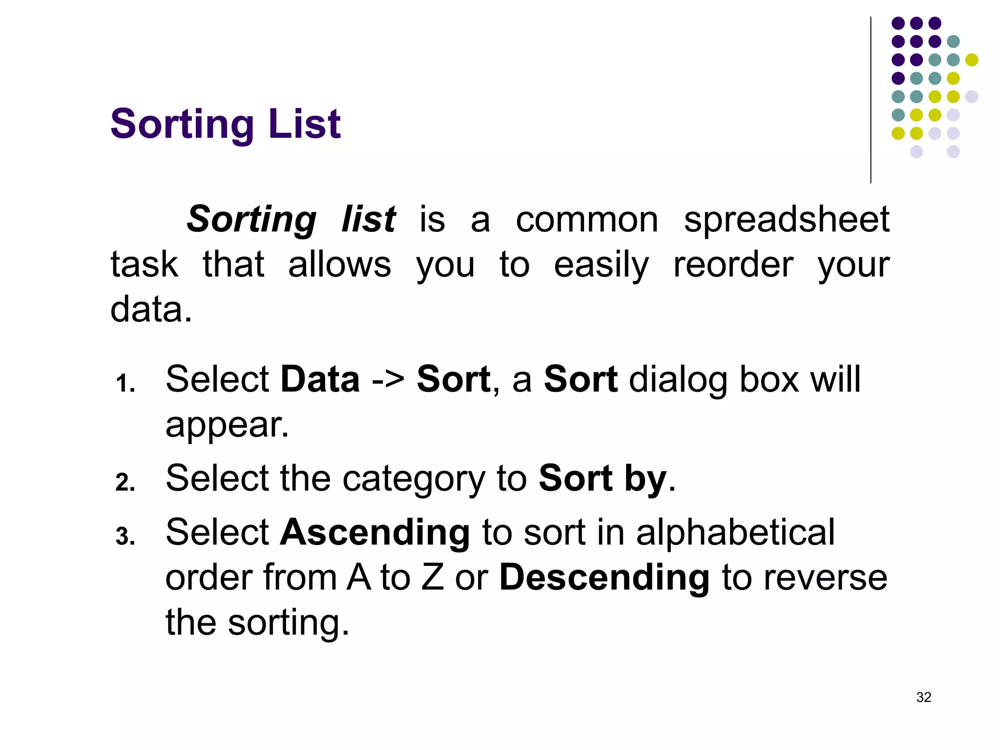
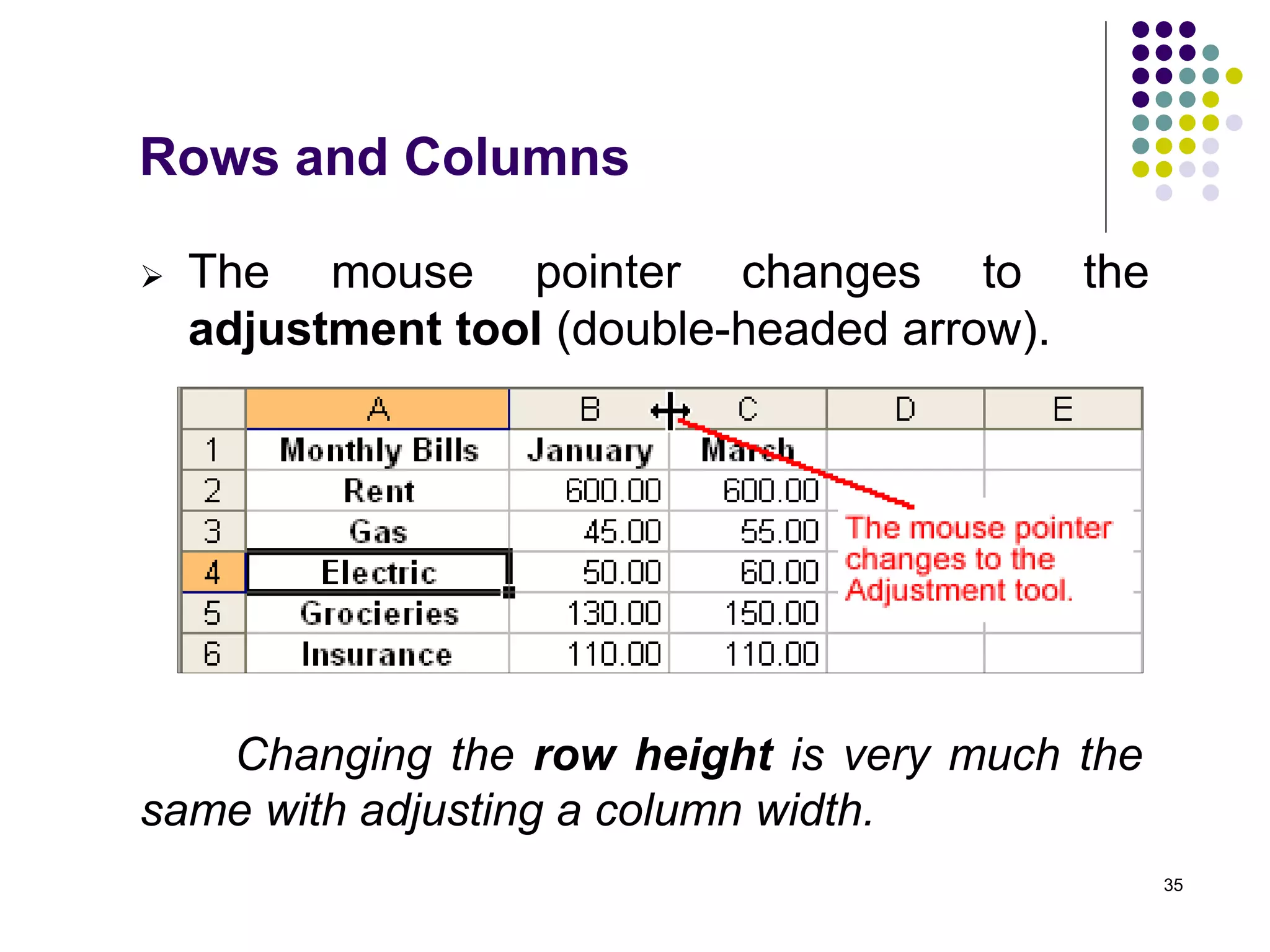
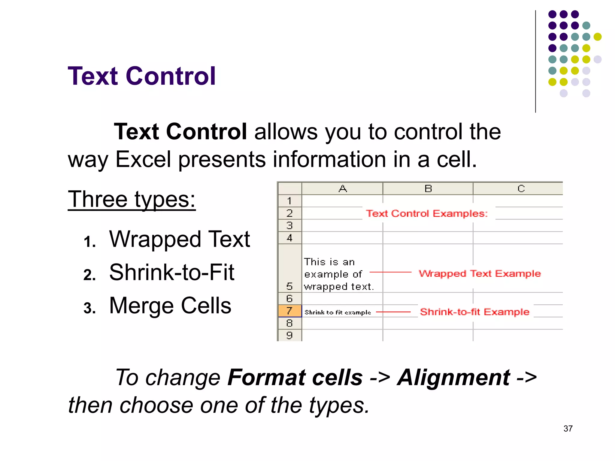
This document provides an overview of Microsoft Excel, including its basic components and functions. It discusses spreadsheet concepts like workbooks, worksheets, and cells. It explains how to enter text, numbers, and formulas into cells. Common Excel functions are described, as well as formatting options, charts, filtering, sorting, and other features. The document is intended as an introductory guide to getting started with the Excel application.

1. MS Excel

2. 2
Intro to MS Excel
Microsoft Excel is the first spreadsheet
application in the Microsoft Office Suite that
allowed the user to define the appearance of
spreadsheets.
Spreadsheet
- a table of values arranged in rows and
columns where each value can have a
predefined relationship to the other values
that sit in their respective cell.

3. 3
Intro to MS Excel
 formula - the relationship between cells.
 labels - the names of the cells.
Electronic Spreadsheet
A type of an accounting computer software
primarily used to work with numbers and text
for performing mathematical computations on a
spreadsheet.
It involves the following:

4. 4
An electronic spreadsheet has the
following purpose:
1. Help organize information, like alphabetizing
a list of names or ordering records, or
Intro to MS Excel
2. Calculate and analyze information using
mathematical formulas.

5. 5
Intro to MS Excel
Advantages:
 It has intelligent cell recomputation.
 Excel allows large numbers of calculations to
be carried out simultaneously.
 It also has extensive graphing capabilities,
and enables users to perform mail merge.

6. 6
Workbook
- This is also called a spreadsheet and a
unique file created by Excel.
- automatically shows in the workspace when
you open Microsoft Excel .
- each workbook contains three worksheets
(labeled Sheet1, Sheet2, and Sheet3).
MS Excel
- a workbook must contain at least one
worksheet.

7. 7
Worksheet - a grid of cells, consisting of
65,536 rows by 256 columns.
Sheet Tabs - separate a workbook into specific
worksheets.
Navigation buttons - allow you to move to
another worksheet in an Excel workbook
and is used to display the first, previous,
next or last worksheets in the workbook.
MS Excel

8. 8
Column headings - contains 256 columns
referenced by alphabetic characters in the
gray boxes that run across the Excel
screen beginning with Column A and
ending with Column IV.
Row headings - contains 65,536 rows
referenced by numbers appearing on the
left and then run down the Excel screen
starting from first row (row 1) to the last
row (row 65536).
MS Excel

9. Chap 5: MS EXCEL 2003 9
MS Excel

10. 10
Name box - shows the address of the current
selection or active cell.
Formula bar - displays information being
entered as you type-in the current or active
cell.
Cells - little boxes that are formed from the
intersection of columns and rows.
The contents of a cell can also be
edited in the Formula bar.
MS Excel

11. 11
Cell address - name designated to each cell
which is comprised of two parts:
a) the column letter; and
b) the row number.
Active cell - refers to the cell that can be acted
upon or receives the data or command you
give it which reveals a dark border.
All other cells reveal a light gray
border.
MS Excel

12. 12
Each cell has a
unique cell address
(i.e. the cell address of
the selected cell is
B3).
MS Excel
cell pointer - the
heavy or darkened
border around the
selected cell.

13. 13
Different spreadsheet information can be
entered into a cell such as text, numbers or
mathematical formulas.
 Text - any entry that is not a number or
formula.
MS Excel
 Numbers - values used when making
calculations.
 Formulas - mathematical calculations.

14. 14
Entering Data in the Cell:
This can be done by clicking on the cell
where you want to type the information.
An insertion point appears in the cell as
the data is typed.
The data being typed appear both in the
active cell or in the Formula bar.
MS Excel

15. 15
Editing Information in the Cell:
Method 1: Direct Cell Editing
This can be done by double-clicking
on the cell that contains the information to be
changed.
Method 2: Formula Bar Editing
This can be done by single clicking on
the cell that contains the information and edit
it in the formula bar.
MS Excel

16. 16
Creating Simple Formula (MDAS Operation):
Step 1: Click the cell where the formula will be
defined.
Step 2: Type the equal sign (=) to let Excel
know a formula is being defined.
Step 3: Type the first number to be included in
the operation.
If it involves numeric value
contained in another cell, click the cell
in which the number is contained.
Using Formula

17. 17
Creating Simple Formula (MDAS Operation):
Step 4: Type the mathematical operator/s (*,
/, +, -) to let Excel know that an
operation is to be performed.
Step 5: Type the second number to be
included in the operation the way it is
done in step 2 especially if it involves
a number in another cell.
Step 6: Press Enter to complete the formula.
Using Formula

18. 18
Creating Complex Formulas:
Simple formulas have one mathematical
operation.
Check Point!
The order of mathematical operations is
very important especially in dealing with
complex formula.
Using Formula
Complex formulas involve more than one
mathematical operation.

19. 19
Order of operations in Complex Formula:
1. Operations enclosed in parenthesis.
Using Formula
2. Exponential calculations (to the power of).
3. Multiplication and division, whichever comes
first.
4. Addition and subtraction, whichever comes
first.

20. 20
Using Formula

21. 21
Applying Formulas to other Cells:
Formula are essential element in using
Excel especially when your dealing with a
range of cells in a given column or row.
Two ways to apply formula to other cells:
1. Copy and Paste Method
2. Fill Formula Method
Using Formula

22. 22
Copy and Paste Formula Method
The process to copy and paste a formula
is identical to that process used to copy and
paste text.
Step 1: Select the cell that contains the
formula to be copied.
Step 2: Click the Copy button.
Marching "ants" appear around
the copied cell(s).
Using Formula

23. 23
Copy and Paste Formula Method
Using Formula

24. 24
Copy and Paste Formula Method
Step 3: Select the cell where the copied
formula is to be pasted.
Step 4: Press the Enter key. The formula is
copied to the new location.
Using Formula

25. 25
Fill Formula Method
- allows you to copy a formula and fill it into
many different consecutive cells at the same
time.
Fill Handle
Using Formula

26. 26
Using the Fill Handle:
Step 1: Click on the cell that contains the
formula to be copied.
Step 2: Position the mouse pointer over the
fill handle.
Step 3: Click and hold the left mouse button,
and then drag the contents to the cell
that's to receive the fill formula.
Step 4: Release the mouse button
Using Formula

27. 27
Conditional formatting allows Excel to
apply a defined format to cells that meet
specific criteria.
Its main goal is to make important cells
stand out so you can find them easier.
Conditional Formatting
These format might include a different
background color, font color or border.

28. 28
Two Methods:
1. Cell Value Is
2. Formula Is
Syntax: =IF(Op1 Operator Op2,True,False)
Example: =IF(B9 > B8,True,False)
You could apply conditional formatting to a
row or column.
Conditional Formatting

29. 29
 Cell Value Is
The simplest method is to have Excel
apply the conditional formatting if the cell
meets a certain criteria.
When using this method, you’re allowed up
to three conditions.
Conditional Formatting

30. 30
 Formula Is
Excel also allows you to use formulas for
conditional formatting.
Benefits of using formulas:
2. It is very useful in doing comparative
analysis as you can color code items that
fall above or below certain ranges.
1. It can reference the values in another cell.
Conditional Formatting

31. 31
Autofilter is a feature that makes
temporarily hiding of data in a spreadsheet very
easy and allows you to focus on specific
spreadsheet entries.
1. Select Data -> Filter, then AutoFilter.
2. Click the drop-down arrow next to the
heading you would like to filter.
3. Click the drop-down arrow again and select
All to display all of the original data.
Autofilter

32. 32
Sorting list is a common spreadsheet
task that allows you to easily reorder your
data.
1. Select Data -> Sort, a Sort dialog box will
appear.
2. Select the category to Sort by.
3. Select Ascending to sort in alphabetical
order from A to Z or Descending to reverse
the sorting.
Sorting List

33. 33
In Excel, you can insert a row or column
anywhere you need it.
Rows and Columns
 A new row is inserted above the cell(s) you
originally selected .
 A new column is inserted to the left of the
existing column.
By default, Excel's columns are 8.43
characters wide, but each individual column
can be enlarged to 240 characters wide.

34. 34
Rows and Columns
You can adjust column width manually or
use AutoFit.
 To access AutoFit choose Format >
Column > AutoFit > Selection.
 To manually adjust the column width, place
your mouse pointer to the right side of the
gray column header.

35. 35
Rows and Columns
 The mouse pointer changes to the
adjustment tool (double-headed arrow).
Changing the row height is very much the
same with adjusting a column width.

36. 36
Rows and Columns
 Drag the Adjustment tool left or right to the
desired width and release the mouse button,
 Double-click the column header border.
Two ways to manually adjust the column width:
Excel "AutoFits" the column, making the
entire column slightly larger than the largest
entry contained in it.

37. 37
Text Control
Text Control allows you to control the
way Excel presents information in a cell.
To change Format cells -> Alignment ->
then choose one of the types.
1. Wrapped Text
2. Shrink-to-Fit
3. Merge Cells
Three types:

38. 38
Text Control
Wrapped Text - wraps the contents of a cell
across several lines if it's too large than the
column width. It increases the height of the
cell as well.
Shrink-to-Fit - shrinks the text so it fits into the
cell; the more text in the cell the smaller it
will appear in the cell.
Merge Cells - can be applied using the Merge
and Center button on the standard toolbar.

39. 39
Text Orientation
Text Orientation is another type of cell
alignment in the Format Cells dialog box which
allows text to be oriented 90 degrees in either
direction up or down.

40. 40
Text Orientation
To Change Text Orientation:
 Select a cell or cell range then choose
Format Cells from the menu bar (Format
Cells dialog box opens).
 Click the Alignment tab.
 Increase or decrease the number shown in
the Degrees field or spin box.
 Click the OK button.

41. 41
SUM - adds a range of cells together.
AVERAGE - calculates the average of a range of
cells.
COUNT - counts the number of chosen data in a
range of cells.
MAX - identifies the largest number in a range of
cells.
Commonly Used Functions

42. 42
MIN - identifies the smallest number in a range of
cells.
COUNTIF - counts the number of cells within a
range that meet the given condition.
ROUND – rounds a number to a specified number
of digits.
Commonly Used Functions
IF - checks whether a condition’s met and returns
a value if True, and another value if false.

43. 43
The Chart Toolbar
Charts can be created in a number of ways
and the quickest way to create and edit your
charts is to use the Chart Toolbar.
Chart Objects List Box - lets you select
different parts of a chart for editing.

44. 44
Chart Types
Excel allows you to create many different
kinds of charts.
Area chart - emphasizes the trend of each
value over time.
It also shows the relationship of parts to
a whole.
Column chart - uses vertical bars or columns
to display values over different categories.
They are excellent at showing
variations in value over time.

45. 45
Chart Types
Bar chart is similar to a column chart except
these use horizontal instead of vertical bars.
Like the column chart, the bar chart
shows variations in value over time.
Line chart shows trends and variations in data
over time.
This type of chart displays a series of
points that are connected over time.

46. 46
Chart Types
Pie chart displays the contribution of each
value to the total.
It’s a very effective way to display
information in representing different parts of
the whole, or the percentages of a total.
Other charts in Excel:
 Doughnut  Stock  Bubble
 XY (scatter)  Radar  Surface
 Cylinder  Cone  Pyramid.

47. 47
Parts of a Chart
Source Data - the range of cells that make up
a chart.
The chart is updated automatically
whenever the information in these cells
change.
Title - the title of the chart.
Legend - the chart key, which identifies each
color on the chart represents.

48. 48
Parts of a Chart
Axis - vertical and horizontal parts of a chart.
Vertical axis - the Y axis,
Horizontal axis - the X axis.
Data Series - the actual charted values,
usually rows or columns of the source data.
Value Axis - the axis that represents the
values or units of the source data.
Category Axis - the axis identifying each data
series.

49. 49
End
Click to add subtitle