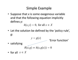
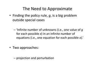
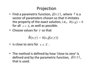
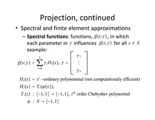
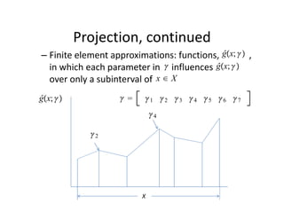
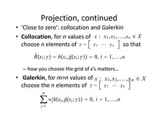
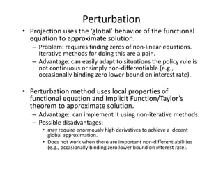
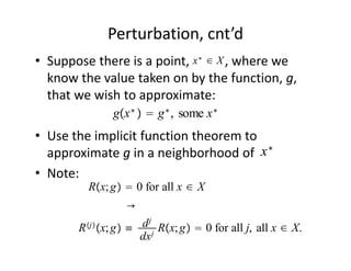
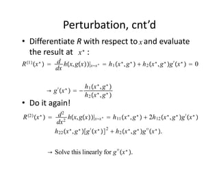
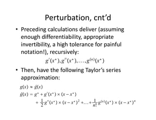
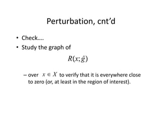
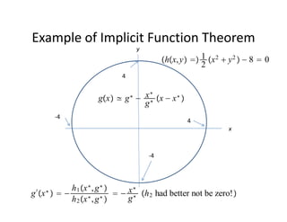
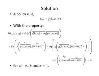
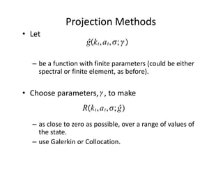
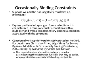
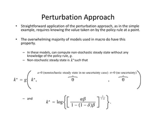
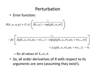
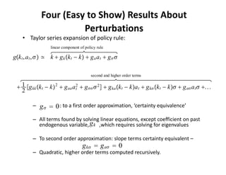
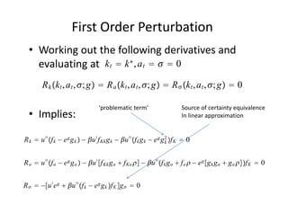
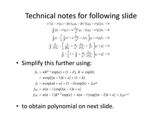
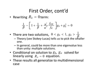
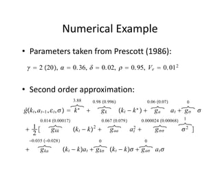
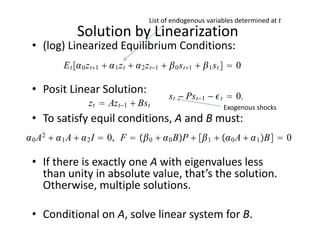
SlideShare a Scribd company logo
Solution Methods for DSGE Models 
and Applications using Linearization

        Lawrence J. Christiano
Overall Outline
• Perturbation and Projection Methods for DSGE 
  Models: an Overview

• Simple New Keynesian model
   – Formulation and log‐linear solution.
   – Ramsey‐optimal policy.
   – Using Dynare to solve the model by log‐linearization:
      • Taylor principle, implications of working capital, News shocks, 
        monetary policy with the long rate.

• Financial Frictions as in BGG
   – Risk shocks and the CKM critique of intertemporal shocks.
   – Dynare exercise.

• Ramsey Optimal Policy, Time Consistency, Timeless 
  Perspective.
Perturbation and Projection 
Methods for Solving DSGE Models
       Lawrence J. Christiano
Outline
• A Simple Example to Illustrate the basic ideas.
  – Functional form characterization of model 
    solution.
  – Use of Projections and Perturbations.

• Neoclassical model.
  – Projection methods
  – Perturbation methods
     • Make sense of the proposition, ‘to a first order 
       approximation, can replace equilibrium conditions with 
       linear expansion about nonstochastic steady state and 
       solve the resulting system using certainty equivalence’ 
Simple Example
• Suppose that x is some exogenous variable 
  and that the following equation implicitly 
  defines y:
               hx, y  0, for all x ∈ X
• Let the solution be defined by the ‘policy rule’, 
  g:
                     y  gx
                                      ‘Error function’
• satisfying
               Rx; g ≡ hx, gx  0
• for all  x ∈ X
The Need to Approximate
• Finding the policy rule, g, is a big problem 
  outside special cases

  – ‘Infinite number of unknowns (i.e., one value of g
    for each possible x) in an infinite number of 
    equations (i.e., one equation for each possible x).’


• Two approaches: 

  – projection and perturbation 
Projection
                                 ĝx;            
• Find a parametric function,             , where     is a 
  vector of parameters chosen so that it imitates 
                                               Rx; g  0
  the property of the exact solution, i.e.,                     
  for all x ∈ X , as well as possible. 
                       
• Choose values for     so that    
                 ̂
                 Rx;   hx, ĝx; 
                        x∈X
• is close to zero for             .

• The method is defined by how ‘close to zero’ is 
                                           ĝx; 
  defined and by the parametric function,              , 
  that is used.
Projection, continued
• Spectral and finite element approximations
                                   ĝx; 
  – Spectral functions: functions,            , in which 
                                      ĝx;             x∈X
    each parameter in     influences              for all            
    example:     
             n                  1
ĝx;     ∑  i Hi x,      
            i0
                                n
 H i x  x i ~ordinary polynominal (not computationaly efficient)
 H i x  T i x,
 T i z : −1, 1 → −1, 1, i th order Chebyshev polynomial
      : X → −1, 1
Projection, continued
                                               ĝx; 
– Finite element approximations: functions,             , 
                                           ĝx; 
  in which each parameter in     influences              
  over only a subinterval of  x ∈ X
ĝx;                    1 2 3 4 5 6 7
                               4

             2


                           X
Projection, continued 
• ‘Close to zero’: collocation and Galerkin
                                  x : x1 , x2 , . . . , xn ∈ X
• Collocation, for n values of                                   
                            1  n
  choose n elements of                                so that   
         ̂
         Rx i ;   hx i , ĝx i ;   0, i  1, . . . , n

   – how you choose the grid of x’s matters…
• Galerkin, for m>n values of                                     
                               x : x1 , x2 , . . . , xm ∈ X
  choose the n elements of      1   n
             m

            ∑ wij hxj , ĝxj ;   0, i  1, . . . , n
             j1
Perturbation
• Projection uses the ‘global’ behavior of the functional 
  equation to approximate solution.
   – Problem: requires finding zeros of non‐linear equations. 
     Iterative methods for doing this are a pain.
   – Advantage: can easily adapt to situations the policy rule is 
     not continuous or simply non‐differentiable (e.g., 
     occasionally binding zero lower bound on interest rate).

• Perturbation method uses local properties of 
  functional equation and Implicit Function/Taylor’s 
  theorem to approximate solution.
   – Advantage:  can implement it using non‐iterative methods. 
   – Possible disadvantages: 
      • may require enormously high derivatives to achieve a  decent 
        global approximation.
      • Does not work when there are important non‐differentiabilities
        (e.g., occasionally binding zero lower bound on interest rate).
Perturbation, cnt’d
                            x∗ ∈ X
• Suppose there is a point,           , where we 
  know the value taken on by the function, g, 
  that we wish to approximate:
               gx ∗   g ∗ , some x ∗
• Use the implicit function theorem to 
  approximate g in a neighborhood of  x ∗
• Note:
          Rx; g  0 for all x ∈ X
                  →
         j
        R x; g ≡ d j Rx; g  0 for all j, all x ∈ X.
                   dx j
Perturbation, cnt’d
• Differentiate R with respect to   and evaluate 
                                  x
                  x∗
  the result at       :
R 1 x ∗   d hx, gx|xx ∗  h 1 x ∗ , g ∗   h 2 x ∗ , g ∗ g ′ x ∗   0
               dx


                 ′   ∗   h 1 x ∗ , g ∗ 
            → g x   −
                         h 2 x ∗ , g ∗ 
• Do it again!
  2
R x  ∗ d 2 hx, gx| ∗  h x ∗ , g ∗   2h x ∗ , g ∗ g ′ x ∗ 
                                xx        11                      12
          dx  2

         h 22 x ∗ , g ∗ g ′ x ∗  2  h 2 x ∗ , g ∗ g ′′ x ∗ .


            → Solve this linearly for g ′′ x ∗ .
Perturbation, cnt’d
• Preceding calculations deliver (assuming 
  enough differentiability, appropriate 
  invertibility, a high tolerance for painful 
  notation!), recursively:
                 g ′ x ∗ , g ′′ x ∗ , . . . , g n x ∗ 
• Then, have the following Taylor’s series 
  approximation:
 gx ≈ ĝx
 ĝx  g ∗  g ′ x ∗   x − x ∗ 
         1 g ′′ x ∗   x − x ∗  2 . . .  1 g n x ∗   x − x ∗  n
            2                                   n!
Perturbation, cnt’d
• Check….
• Study the graph of
                        Rx; ĝ

           x∈X
  – over                to verify that it is everywhere close 
    to zero (or, at least in the region of interest). 
Example of Implicit Function Theorem
                                     y
                                              hx, y  1 x 2  y 2  − 8  0
                                                          2
                                4


                       gx ≃   g∗     x ∗ x − x ∗ 
                                     − ∗
                                      g
           ‐4
                                                        4
                                                                   x


                                         ‐4


              h 1 x ∗ , g ∗    x ∗ h 2 had better not be zero!
g′     ∗
     x   −                  − ∗
                     ∗ ∗
              h 2 x , g        g
Neoclassical Growth Model
• Objective:
                                                1−
                                            c −1
               E 0 ∑  t uc t , uc t   t
                                             1−
                  t0

• Constraints:
            c t  expk t1  ≤ fk t , a t , t  0, 1, 2, . . . .


                a t  a t−1   t .


         fk t , a t   expk t  expa t   1 −  expk t .
Efficiency Condition
                     ct1

E t u ′ fk t , a t  − expk t1 

                                ct1                period t1 marginal product of capital

    − u ′ fk t1 , a t   t1  − expk t2          f K k t1 , a t   t1       0.

 • Here,                    k t , a t ~given numbers
                             t1 ~ iid, mean zero variance V 
                            time t choice variable, k t1

 • Convenient to suppose the model is the limit 
                             →1                     
   of a sequence of models,             , indexed by   
                                 t1 ~ 2 V  ,   1.
Solution
   • A policy rule,
                                             k t1  gk t , a t , .

   • With the property:
                                                  ct

Rk t , a t , ; g ≡ E t u ′ fk t , a t  − expgk t , a t , 

                                                            ct1

                     k t1           a t1                                 k t1           a t1

 − u ′     f gk t , a t , , a t   t1          − exp g gk t , a t , , a t   t1 , 


                                                                            k t1           a t1

                                                              fK      gk t , a t , , a t   t1     0,

   • for all   a t , k t and   1.
Projection Methods
• Let                     
                              ĝk t , a t , ; 

    – be a function with finite parameters (could be either 
      spectral or finite element, as before).

                    
• Choose parameters,   , to make
                             Rk t , a t , ; ĝ
    – as close to zero as possible, over a range of values of 
      the state.
    – use Galerkin or Collocation. 
Occasionally Binding Constraints
• Suppose we add the non‐negativity constraint on 
  investment:
          expgk t , a t ,  − 1 −  expk t  ≥ 0
• Express problem in Lagrangian form and optimum is 
  characterized in terms of equality conditions with a 
  multiplier and with a complementary slackness condition 
  associated with the constraint.

• Conceptually straightforward to apply preceding method. 
  For details, see Christiano‐Fisher, ‘Algorithms for Solving 
  Dynamic Models with Occasionally Binding Constraints’, 
  2000, Journal of Economic Dynamics and Control.
   – This paper describes alternative strategies, based on 
     parameterizing the expectation function, that may be easier, 
     when constraints are occasionally binding constraints.
Perturbation Approach
•   Straightforward application of the perturbation approach, as in the simple 
    example, requires knowing the value taken on by the policy rule at a point.

•   The overwhelming majority of models used in macro do have this 
    property. 

     – In these models, can compute non‐stochastic steady state without any 
       knowledge of the policy rule, g.
                                       k∗
     – Non‐stochastic steady state is      such that


                a0 (nonstochastic steady state in no uncertainty case) 0 (no uncertainty)
∗           ∗
                                                                             
k g k ,                               0                              ,       0


                                                                 1
     – and                                                    1−
                      k∗    log                                          .
                                         1 − 1 − 
Perturbation
    • Error function:
                                                 ct

Rk t , a t , ; g ≡ E t u ′ fk t , a t  − expgk t , a t , 


                                                       ct1

  − u ′ fgk t , a t , , a t   t1  − expggk t , a t , , a t   t1 , 

                                                       f K gk t , a t , , a t   t1   0,

                              k t , a t , .
         – for all values of                
    • So, all order derivatives of R with respect to its 
      arguments are zero (assuming they exist!).
Four (Easy to Show) Results About 
                        Perturbations
    • Taylor series expansion of policy rule:
                   linear component of policy rule

gk t , a t ,  ≃ k  g k k t − k  g a a t  g  

                                          second and higher order terms

  1 g kk k t − k 2  g aa a 2  g   2   g ka k t − ka t  g k k t − k  g a a t  . . .
                                t
   2

          –   g   0 : to a first order approximation, ‘certainty equivalence’ 
          – All terms found by solving linear equations, except coefficient on past 
                                  gk
            endogenous variable,        ,which requires solving for eigenvalues

          – To second order approximation: slope terms certainty equivalent –
                                     g k  g a  0
          – Quadratic, higher order terms computed recursively.
First Order Perturbation
  • Working out the following derivatives and 
    evaluating at  k t  k ∗ , a t    0
        R k k t , a t , ; g  R a k t , a t , ; g  R  k t , a t , ; g  0

                                   ‘problematic term’                      Source of certainty equivalence
  • Implies:                                                               In linear approximation


R k  u ′′ f k − e g g k  − u ′ f Kk g k − u ′′ f k g k − e g g 2 f K  0
                                                                     k


R a  u ′′ f a − e g g a  − u ′ f Kk g a  f Ka  − u ′′ f k g a  f a  − e g g k g a  g a f K  0


R   −u ′ e g  u ′′ f k − e g g k f K g   0
Technical notes for following slide
               u ′′ f k − e g g k  − u ′ f Kk g k − u ′′ f k g k − e g g 2 f K
                                                                              k        0
                       1 f − e g g  − u ′ f Kk g − f g − e g g 2 f K               0
                        k            k
                                                 u ′′
                                                        k       k k           k

                       1 f − 1 e g  u ′ f Kk  f f K g  e g g 2 f K                  0
                        k                       u ′′
                                                             k       k          k


                  1 fk −               1  u ′ f Kk  f k g  g 2                      0
                                                                           k
                   eg fK             f K       u ′′ e g f K      eg              k


                                1 − 1  1  u ′ f Kk                     gk  g2  0
                                                                               k
                                          u ′′ e g f K

• Simplify this further using:
       f K  K−1 expa  1 − , K ≡ expk
            exp − 1k  a  1 − 
       f k   expk  a  1 −  expk  f K e g
      f Kk   − 1 exp − 1k  a
      f KK   − 1K−2 expa   − 1 exp − 2k  a  f Kk e −g


• to obtain polynomial on next slide. 
First Order, cont’d
             Rk  0
• Rewriting                term:
           1 − 1  1  u ′ f KK          gk  g2  0
                                             k
                       u ′′ f K

                            0  g k  1, g k  1
• There are two solutions,                                   
                                                            
   – Theory (see Stokey‐Lucas) tells us to pick the smaller 
     one. 
   – In general, could be more than one eigenvalue less 
     than unity: multiple solutions.
                                    gk ga
• Conditional on solution to     ,         solved for 
                  Ra  0
  linearly using                equation.
• These results all generalize to multidimensional 
  case
Numerical Example
• Parameters taken from Prescott (1986):
   2 20,   0. 36,   0. 02,   0. 95, Ve  0. 01 2


• Second order approximation:
                           3.88    0.98 0.996                          0.06 0.07         0
                                                                              
ĝk t , a t−1 ,  t ,   k ∗        gk          k t − k ∗           ga at  g 
         0.014 0.00017                   0.067 0.079            0.000024 0.00068   1
                                                                                    
 1         g kk          k t − k  g aa
                                   2
                                                           a2
                                                            t              g        2 
  2
    −0.035 −0.028                    0                             0
                                                    
       g ka          k t − ka t  g k k t − k  g a a t 
Conclusion
• For modest US‐sized fluctuations and for 
  aggregate quantities, it is reasonable to work 
  with first order perturbations.

• First order perturbation: linearize (or, log‐
  linearize) equilibrium conditions around non‐
  stochastic steady state and solve the resulting 
  system. 
   – This approach assumes ‘certainty equivalence’. Ok, as 
     a first order approximation.
List of endogenous variables determined at t
              Solution by Linearization
 • (log) Linearized Equilibrium Conditions:
          E t  0 z t1   1 z t   2 z t−1   0 s t1   1 s t   0

 • Posit Linear Solution:
                                                s t − Ps t−1 −  t  0.
                   z t  Az t−1  Bs t                             Exogenous shocks
 • To satisfy equil conditions, A and B must:
 0 A2   1 A   2 I  0, F   0   0 BP   1   0 A   1 B  0

 • If there is exactly one A with eigenvalues less 
   than unity in absolute value, that’s the solution. 
   Otherwise, multiple solutions.

 • Conditional on A, solve linear system for B. 

More Related Content

What's hot

Random Matrix Theory and Machine Learning - Part 2
Random Matrix Theory and Machine Learning - Part 2Random Matrix Theory and Machine Learning - Part 2
Random Matrix Theory and Machine Learning - Part 2
Fabian Pedregosa
 
Random Matrix Theory and Machine Learning - Part 3
Random Matrix Theory and Machine Learning - Part 3Random Matrix Theory and Machine Learning - Part 3
Random Matrix Theory and Machine Learning - Part 3
Fabian Pedregosa
 
Random Matrix Theory and Machine Learning - Part 1
Random Matrix Theory and Machine Learning - Part 1Random Matrix Theory and Machine Learning - Part 1
Random Matrix Theory and Machine Learning - Part 1
Fabian Pedregosa
 
Application of the Monte-Carlo Method to Nonlinear Stochastic Optimization wi...
Application of the Monte-Carlo Method to Nonlinear Stochastic Optimization wi...Application of the Monte-Carlo Method to Nonlinear Stochastic Optimization wi...
Application of the Monte-Carlo Method to Nonlinear Stochastic Optimization wi...
SSA KPI
 
Savage-Dickey paradox
Savage-Dickey paradoxSavage-Dickey paradox
Savage-Dickey paradox
Christian Robert
 
Welcome to International Journal of Engineering Research and Development (IJERD)
Welcome to International Journal of Engineering Research and Development (IJERD)Welcome to International Journal of Engineering Research and Development (IJERD)
Welcome to International Journal of Engineering Research and Development (IJERD)
IJERD Editor
 
Discrete Probability Distributions
Discrete  Probability DistributionsDiscrete  Probability Distributions
Discrete Probability Distributions
E-tan
 
Tensor Decomposition and its Applications
Tensor Decomposition and its ApplicationsTensor Decomposition and its Applications
Tensor Decomposition and its Applications
Keisuke OTAKI
 
Lesson 15: Exponential Growth and Decay
Lesson 15: Exponential Growth and DecayLesson 15: Exponential Growth and Decay
Lesson 15: Exponential Growth and Decay
Matthew Leingang
 
1 - Linear Regression
1 - Linear Regression1 - Linear Regression
1 - Linear Regression
Nikita Zhiltsov
 
Lesson 16: Inverse Trigonometric Functions
Lesson 16: Inverse Trigonometric FunctionsLesson 16: Inverse Trigonometric Functions
Lesson 16: Inverse Trigonometric Functions
Matthew Leingang
 
Numerical solution of boundary value problems by piecewise analysis method
Numerical solution of boundary value problems by piecewise analysis methodNumerical solution of boundary value problems by piecewise analysis method
Numerical solution of boundary value problems by piecewise analysis method
Alexander Decker
 
MCQMC 2020 talk: Importance Sampling for a Robust and Efficient Multilevel Mo...
MCQMC 2020 talk: Importance Sampling for a Robust and Efficient Multilevel Mo...MCQMC 2020 talk: Importance Sampling for a Robust and Efficient Multilevel Mo...
MCQMC 2020 talk: Importance Sampling for a Robust and Efficient Multilevel Mo...
Chiheb Ben Hammouda
 
Rouviere
RouviereRouviere
Rouviere
eric_gautier
 
Seminar Talk: Multilevel Hybrid Split Step Implicit Tau-Leap for Stochastic R...
Seminar Talk: Multilevel Hybrid Split Step Implicit Tau-Leap for Stochastic R...Seminar Talk: Multilevel Hybrid Split Step Implicit Tau-Leap for Stochastic R...
Seminar Talk: Multilevel Hybrid Split Step Implicit Tau-Leap for Stochastic R...
Chiheb Ben Hammouda
 
Numerical smoothing and hierarchical approximations for efficient option pric...
Numerical smoothing and hierarchical approximations for efficient option pric...Numerical smoothing and hierarchical approximations for efficient option pric...
Numerical smoothing and hierarchical approximations for efficient option pric...
Chiheb Ben Hammouda
 
STUDIES ON INTUTIONISTIC FUZZY INFORMATION MEASURE
STUDIES ON INTUTIONISTIC FUZZY INFORMATION MEASURESTUDIES ON INTUTIONISTIC FUZZY INFORMATION MEASURE
STUDIES ON INTUTIONISTIC FUZZY INFORMATION MEASURE
Surender Singh
 
Lesson 14: Derivatives of Logarithmic and Exponential Functions
Lesson 14: Derivatives of Logarithmic and Exponential FunctionsLesson 14: Derivatives of Logarithmic and Exponential Functions
Lesson 14: Derivatives of Logarithmic and Exponential Functions
Matthew Leingang
 
Lecture cochran
Lecture cochranLecture cochran
Lecture cochran
sabbir11
 
Lesson 13: Related Rates Problems
Lesson 13: Related Rates ProblemsLesson 13: Related Rates Problems
Lesson 13: Related Rates Problems
Matthew Leingang
 

What's hot (20)

Random Matrix Theory and Machine Learning - Part 2
Random Matrix Theory and Machine Learning - Part 2Random Matrix Theory and Machine Learning - Part 2
Random Matrix Theory and Machine Learning - Part 2
 
Random Matrix Theory and Machine Learning - Part 3
Random Matrix Theory and Machine Learning - Part 3Random Matrix Theory and Machine Learning - Part 3
Random Matrix Theory and Machine Learning - Part 3
 
Random Matrix Theory and Machine Learning - Part 1
Random Matrix Theory and Machine Learning - Part 1Random Matrix Theory and Machine Learning - Part 1
Random Matrix Theory and Machine Learning - Part 1
 
Application of the Monte-Carlo Method to Nonlinear Stochastic Optimization wi...
Application of the Monte-Carlo Method to Nonlinear Stochastic Optimization wi...Application of the Monte-Carlo Method to Nonlinear Stochastic Optimization wi...
Application of the Monte-Carlo Method to Nonlinear Stochastic Optimization wi...
 
Savage-Dickey paradox
Savage-Dickey paradoxSavage-Dickey paradox
Savage-Dickey paradox
 
Welcome to International Journal of Engineering Research and Development (IJERD)
Welcome to International Journal of Engineering Research and Development (IJERD)Welcome to International Journal of Engineering Research and Development (IJERD)
Welcome to International Journal of Engineering Research and Development (IJERD)
 
Discrete Probability Distributions
Discrete  Probability DistributionsDiscrete  Probability Distributions
Discrete Probability Distributions
 
Tensor Decomposition and its Applications
Tensor Decomposition and its ApplicationsTensor Decomposition and its Applications
Tensor Decomposition and its Applications
 
Lesson 15: Exponential Growth and Decay
Lesson 15: Exponential Growth and DecayLesson 15: Exponential Growth and Decay
Lesson 15: Exponential Growth and Decay
 
1 - Linear Regression
1 - Linear Regression1 - Linear Regression
1 - Linear Regression
 
Lesson 16: Inverse Trigonometric Functions
Lesson 16: Inverse Trigonometric FunctionsLesson 16: Inverse Trigonometric Functions
Lesson 16: Inverse Trigonometric Functions
 
Numerical solution of boundary value problems by piecewise analysis method
Numerical solution of boundary value problems by piecewise analysis methodNumerical solution of boundary value problems by piecewise analysis method
Numerical solution of boundary value problems by piecewise analysis method
 
MCQMC 2020 talk: Importance Sampling for a Robust and Efficient Multilevel Mo...
MCQMC 2020 talk: Importance Sampling for a Robust and Efficient Multilevel Mo...MCQMC 2020 talk: Importance Sampling for a Robust and Efficient Multilevel Mo...
MCQMC 2020 talk: Importance Sampling for a Robust and Efficient Multilevel Mo...
 
Rouviere
RouviereRouviere
Rouviere
 
Seminar Talk: Multilevel Hybrid Split Step Implicit Tau-Leap for Stochastic R...
Seminar Talk: Multilevel Hybrid Split Step Implicit Tau-Leap for Stochastic R...Seminar Talk: Multilevel Hybrid Split Step Implicit Tau-Leap for Stochastic R...
Seminar Talk: Multilevel Hybrid Split Step Implicit Tau-Leap for Stochastic R...
 
Numerical smoothing and hierarchical approximations for efficient option pric...
Numerical smoothing and hierarchical approximations for efficient option pric...Numerical smoothing and hierarchical approximations for efficient option pric...
Numerical smoothing and hierarchical approximations for efficient option pric...
 
STUDIES ON INTUTIONISTIC FUZZY INFORMATION MEASURE
STUDIES ON INTUTIONISTIC FUZZY INFORMATION MEASURESTUDIES ON INTUTIONISTIC FUZZY INFORMATION MEASURE
STUDIES ON INTUTIONISTIC FUZZY INFORMATION MEASURE
 
Lesson 14: Derivatives of Logarithmic and Exponential Functions
Lesson 14: Derivatives of Logarithmic and Exponential FunctionsLesson 14: Derivatives of Logarithmic and Exponential Functions
Lesson 14: Derivatives of Logarithmic and Exponential Functions
 
Lecture cochran
Lecture cochranLecture cochran
Lecture cochran
 
Lesson 13: Related Rates Problems
Lesson 13: Related Rates ProblemsLesson 13: Related Rates Problems
Lesson 13: Related Rates Problems
 

Viewers also liked

Lecture on nk [compatibility mode]
Lecture on nk [compatibility mode]Lecture on nk [compatibility mode]
Lecture on nk [compatibility mode]
NBER
 
Csvfrictions
CsvfrictionsCsvfrictions
Csvfrictions
NBER
 
Dynare exercise
Dynare exerciseDynare exercise
Dynare exercise
NBER
 
Optimalpolicyhandout
OptimalpolicyhandoutOptimalpolicyhandout
Optimalpolicyhandout
NBER
 
Applications: Prediction
Applications: PredictionApplications: Prediction
Applications: Prediction
NBER
 
Econometrics of High-Dimensional Sparse Models
Econometrics of High-Dimensional Sparse ModelsEconometrics of High-Dimensional Sparse Models
Econometrics of High-Dimensional Sparse Models
NBER
 
High-Dimensional Methods: Examples for Inference on Structural Effects
High-Dimensional Methods: Examples for Inference on Structural EffectsHigh-Dimensional Methods: Examples for Inference on Structural Effects
High-Dimensional Methods: Examples for Inference on Structural Effects
NBER
 
Big Data Analysis
Big Data AnalysisBig Data Analysis
Big Data Analysis
NBER
 
Nuts and bolts
Nuts and boltsNuts and bolts
Nuts and bolts
NBER
 

Viewers also liked (9)

Lecture on nk [compatibility mode]
Lecture on nk [compatibility mode]Lecture on nk [compatibility mode]
Lecture on nk [compatibility mode]
 
Csvfrictions
CsvfrictionsCsvfrictions
Csvfrictions
 
Dynare exercise
Dynare exerciseDynare exercise
Dynare exercise
 
Optimalpolicyhandout
OptimalpolicyhandoutOptimalpolicyhandout
Optimalpolicyhandout
 
Applications: Prediction
Applications: PredictionApplications: Prediction
Applications: Prediction
 
Econometrics of High-Dimensional Sparse Models
Econometrics of High-Dimensional Sparse ModelsEconometrics of High-Dimensional Sparse Models
Econometrics of High-Dimensional Sparse Models
 
High-Dimensional Methods: Examples for Inference on Structural Effects
High-Dimensional Methods: Examples for Inference on Structural EffectsHigh-Dimensional Methods: Examples for Inference on Structural Effects
High-Dimensional Methods: Examples for Inference on Structural Effects
 
Big Data Analysis
Big Data AnalysisBig Data Analysis
Big Data Analysis
 
Nuts and bolts
Nuts and boltsNuts and bolts
Nuts and bolts
 

Similar to Lecture on solving1

Monte-Carlo method for Two-Stage SLP
Monte-Carlo method for Two-Stage SLPMonte-Carlo method for Two-Stage SLP
Monte-Carlo method for Two-Stage SLP
SSA KPI
 
B. Sazdovic - Noncommutativity and T-duality
B. Sazdovic - Noncommutativity and T-dualityB. Sazdovic - Noncommutativity and T-duality
B. Sazdovic - Noncommutativity and T-duality
SEENET-MTP
 
Nonlinear Stochastic Programming by the Monte-Carlo method
Nonlinear Stochastic Programming by the Monte-Carlo methodNonlinear Stochastic Programming by the Monte-Carlo method
Nonlinear Stochastic Programming by the Monte-Carlo method
SSA KPI
 
PhD thesis presentation of Nguyen Bich Van
PhD thesis presentation of Nguyen Bich VanPhD thesis presentation of Nguyen Bich Van
PhD thesis presentation of Nguyen Bich Van
Nguyen Bich Van
 
Randomness conductors
Randomness conductorsRandomness conductors
Randomness conductors
wtyru1989
 
Transaction Costs Made Tractable
Transaction Costs Made TractableTransaction Costs Made Tractable
Transaction Costs Made Tractable
guasoni
 
Convex optimization methods
Convex optimization methodsConvex optimization methods
Convex optimization methods
Dong Guo
 
Stochastic Approximation and Simulated Annealing
Stochastic Approximation and Simulated AnnealingStochastic Approximation and Simulated Annealing
Stochastic Approximation and Simulated Annealing
SSA KPI
 
02 newton-raphson
02 newton-raphson02 newton-raphson
02 newton-raphson
stephanus_ananda
 
Ml mle_bayes
Ml  mle_bayesMl  mle_bayes
Ml mle_bayes
Phong Vo
 
stochastic processes-2.ppt
stochastic processes-2.pptstochastic processes-2.ppt
stochastic processes-2.ppt
kjbvhjgcdrxs46d576fu
 
Constrained Maximization
Constrained MaximizationConstrained Maximization
Constrained Maximization
GlennAnthony7
 
Gaussian Integration
Gaussian IntegrationGaussian Integration
Gaussian Integration
Reza Rahimi
 
Options Portfolio Selection
Options Portfolio SelectionOptions Portfolio Selection
Options Portfolio Selection
guasoni
 
Funcion gamma
Funcion gammaFuncion gamma
Funcion gamma
Adhana Hary Wibowo
 
CI_L01_Optimization.pdf
CI_L01_Optimization.pdfCI_L01_Optimization.pdf
CI_L01_Optimization.pdf
SantiagoGarridoBulln
 
Ch02
Ch02Ch02
Ch02
waiwai28
 
Nonlinear Stochastic Optimization by the Monte-Carlo Method
Nonlinear Stochastic Optimization by the Monte-Carlo MethodNonlinear Stochastic Optimization by the Monte-Carlo Method
Nonlinear Stochastic Optimization by the Monte-Carlo Method
SSA KPI
 
Numerical Linear Algebra for Data and Link Analysis.
Numerical Linear Algebra for Data and Link Analysis.Numerical Linear Algebra for Data and Link Analysis.
Numerical Linear Algebra for Data and Link Analysis.
Leonid Zhukov
 
Likelihood survey-nber-0713101
Likelihood survey-nber-0713101Likelihood survey-nber-0713101
Likelihood survey-nber-0713101
NBER
 

Similar to Lecture on solving1 (20)

Monte-Carlo method for Two-Stage SLP
Monte-Carlo method for Two-Stage SLPMonte-Carlo method for Two-Stage SLP
Monte-Carlo method for Two-Stage SLP
 
B. Sazdovic - Noncommutativity and T-duality
B. Sazdovic - Noncommutativity and T-dualityB. Sazdovic - Noncommutativity and T-duality
B. Sazdovic - Noncommutativity and T-duality
 
Nonlinear Stochastic Programming by the Monte-Carlo method
Nonlinear Stochastic Programming by the Monte-Carlo methodNonlinear Stochastic Programming by the Monte-Carlo method
Nonlinear Stochastic Programming by the Monte-Carlo method
 
PhD thesis presentation of Nguyen Bich Van
PhD thesis presentation of Nguyen Bich VanPhD thesis presentation of Nguyen Bich Van
PhD thesis presentation of Nguyen Bich Van
 
Randomness conductors
Randomness conductorsRandomness conductors
Randomness conductors
 
Transaction Costs Made Tractable
Transaction Costs Made TractableTransaction Costs Made Tractable
Transaction Costs Made Tractable
 
Convex optimization methods
Convex optimization methodsConvex optimization methods
Convex optimization methods
 
Stochastic Approximation and Simulated Annealing
Stochastic Approximation and Simulated AnnealingStochastic Approximation and Simulated Annealing
Stochastic Approximation and Simulated Annealing
 
02 newton-raphson
02 newton-raphson02 newton-raphson
02 newton-raphson
 
Ml mle_bayes
Ml  mle_bayesMl  mle_bayes
Ml mle_bayes
 
stochastic processes-2.ppt
stochastic processes-2.pptstochastic processes-2.ppt
stochastic processes-2.ppt
 
Constrained Maximization
Constrained MaximizationConstrained Maximization
Constrained Maximization
 
Gaussian Integration
Gaussian IntegrationGaussian Integration
Gaussian Integration
 
Options Portfolio Selection
Options Portfolio SelectionOptions Portfolio Selection
Options Portfolio Selection
 
Funcion gamma
Funcion gammaFuncion gamma
Funcion gamma
 
CI_L01_Optimization.pdf
CI_L01_Optimization.pdfCI_L01_Optimization.pdf
CI_L01_Optimization.pdf
 
Ch02
Ch02Ch02
Ch02
 
Nonlinear Stochastic Optimization by the Monte-Carlo Method
Nonlinear Stochastic Optimization by the Monte-Carlo MethodNonlinear Stochastic Optimization by the Monte-Carlo Method
Nonlinear Stochastic Optimization by the Monte-Carlo Method
 
Numerical Linear Algebra for Data and Link Analysis.
Numerical Linear Algebra for Data and Link Analysis.Numerical Linear Algebra for Data and Link Analysis.
Numerical Linear Algebra for Data and Link Analysis.
 
Likelihood survey-nber-0713101
Likelihood survey-nber-0713101Likelihood survey-nber-0713101
Likelihood survey-nber-0713101
 

More from NBER

FISCAL STIMULUS IN ECONOMIC UNIONS: WHAT ROLE FOR STATES
FISCAL STIMULUS IN ECONOMIC UNIONS: WHAT ROLE FOR STATESFISCAL STIMULUS IN ECONOMIC UNIONS: WHAT ROLE FOR STATES
FISCAL STIMULUS IN ECONOMIC UNIONS: WHAT ROLE FOR STATES
NBER
 
Business in the United States Who Owns it and How Much Tax They Pay
Business in the United States Who Owns it and How Much Tax They PayBusiness in the United States Who Owns it and How Much Tax They Pay
Business in the United States Who Owns it and How Much Tax They Pay
NBER
 
Redistribution through Minimum Wage Regulation: An Analysis of Program Linkag...
Redistribution through Minimum Wage Regulation: An Analysis of Program Linkag...Redistribution through Minimum Wage Regulation: An Analysis of Program Linkag...
Redistribution through Minimum Wage Regulation: An Analysis of Program Linkag...
NBER
 
The Distributional E ffects of U.S. Clean Energy Tax Credits
The Distributional Effects of U.S. Clean Energy Tax CreditsThe Distributional Effects of U.S. Clean Energy Tax Credits
The Distributional E ffects of U.S. Clean Energy Tax Credits
NBER
 
An Experimental Evaluation of Strategies to Increase Property Tax Compliance:...
An Experimental Evaluation of Strategies to Increase Property Tax Compliance:...An Experimental Evaluation of Strategies to Increase Property Tax Compliance:...
An Experimental Evaluation of Strategies to Increase Property Tax Compliance:...
NBER
 
Nbe rtopicsandrecomvlecture1
Nbe rtopicsandrecomvlecture1Nbe rtopicsandrecomvlecture1
Nbe rtopicsandrecomvlecture1
NBER
 
Nbe rcausalpredictionv111 lecture2
Nbe rcausalpredictionv111 lecture2Nbe rcausalpredictionv111 lecture2
Nbe rcausalpredictionv111 lecture2
NBER
 
Recommenders, Topics, and Text
Recommenders, Topics, and TextRecommenders, Topics, and Text
Recommenders, Topics, and Text
NBER
 
Machine Learning and Causal Inference
Machine Learning and Causal InferenceMachine Learning and Causal Inference
Machine Learning and Causal Inference
NBER
 
Introduction to Supervised ML Concepts and Algorithms
Introduction to Supervised ML Concepts and AlgorithmsIntroduction to Supervised ML Concepts and Algorithms
Introduction to Supervised ML Concepts and Algorithms
NBER
 
Jackson nber-slides2014 lecture3
Jackson nber-slides2014 lecture3Jackson nber-slides2014 lecture3
Jackson nber-slides2014 lecture3
NBER
 
Jackson nber-slides2014 lecture1
Jackson nber-slides2014 lecture1Jackson nber-slides2014 lecture1
Jackson nber-slides2014 lecture1
NBER
 
Acemoglu lecture2
Acemoglu lecture2Acemoglu lecture2
Acemoglu lecture2
NBER
 
Acemoglu lecture4
Acemoglu lecture4Acemoglu lecture4
Acemoglu lecture4
NBER
 
The NBER Working Paper Series at 20,000 - Joshua Gans
The NBER Working Paper Series at 20,000 - Joshua GansThe NBER Working Paper Series at 20,000 - Joshua Gans
The NBER Working Paper Series at 20,000 - Joshua Gans
NBER
 
The NBER Working Paper Series at 20,000 - Claudia Goldin
The NBER Working Paper Series at 20,000 - Claudia GoldinThe NBER Working Paper Series at 20,000 - Claudia Goldin
The NBER Working Paper Series at 20,000 - Claudia Goldin
NBER
 
The NBER Working Paper Series at 20,000 - James Poterba
The NBER Working Paper Series at 20,000 - James PoterbaThe NBER Working Paper Series at 20,000 - James Poterba
The NBER Working Paper Series at 20,000 - James Poterba
NBER
 
The NBER Working Paper Series at 20,000 - Scott Stern
The NBER Working Paper Series at 20,000 - Scott SternThe NBER Working Paper Series at 20,000 - Scott Stern
The NBER Working Paper Series at 20,000 - Scott Stern
NBER
 
The NBER Working Paper Series at 20,000 - Glenn Ellison
The NBER Working Paper Series at 20,000 - Glenn EllisonThe NBER Working Paper Series at 20,000 - Glenn Ellison
The NBER Working Paper Series at 20,000 - Glenn Ellison
NBER
 
L3 1b
L3 1bL3 1b
L3 1b
NBER
 

More from NBER (20)

FISCAL STIMULUS IN ECONOMIC UNIONS: WHAT ROLE FOR STATES
FISCAL STIMULUS IN ECONOMIC UNIONS: WHAT ROLE FOR STATESFISCAL STIMULUS IN ECONOMIC UNIONS: WHAT ROLE FOR STATES
FISCAL STIMULUS IN ECONOMIC UNIONS: WHAT ROLE FOR STATES
 
Business in the United States Who Owns it and How Much Tax They Pay
Business in the United States Who Owns it and How Much Tax They PayBusiness in the United States Who Owns it and How Much Tax They Pay
Business in the United States Who Owns it and How Much Tax They Pay
 
Redistribution through Minimum Wage Regulation: An Analysis of Program Linkag...
Redistribution through Minimum Wage Regulation: An Analysis of Program Linkag...Redistribution through Minimum Wage Regulation: An Analysis of Program Linkag...
Redistribution through Minimum Wage Regulation: An Analysis of Program Linkag...
 
The Distributional E ffects of U.S. Clean Energy Tax Credits
The Distributional Effects of U.S. Clean Energy Tax CreditsThe Distributional Effects of U.S. Clean Energy Tax Credits
The Distributional E ffects of U.S. Clean Energy Tax Credits
 
An Experimental Evaluation of Strategies to Increase Property Tax Compliance:...
An Experimental Evaluation of Strategies to Increase Property Tax Compliance:...An Experimental Evaluation of Strategies to Increase Property Tax Compliance:...
An Experimental Evaluation of Strategies to Increase Property Tax Compliance:...
 
Nbe rtopicsandrecomvlecture1
Nbe rtopicsandrecomvlecture1Nbe rtopicsandrecomvlecture1
Nbe rtopicsandrecomvlecture1
 
Nbe rcausalpredictionv111 lecture2
Nbe rcausalpredictionv111 lecture2Nbe rcausalpredictionv111 lecture2
Nbe rcausalpredictionv111 lecture2
 
Recommenders, Topics, and Text
Recommenders, Topics, and TextRecommenders, Topics, and Text
Recommenders, Topics, and Text
 
Machine Learning and Causal Inference
Machine Learning and Causal InferenceMachine Learning and Causal Inference
Machine Learning and Causal Inference
 
Introduction to Supervised ML Concepts and Algorithms
Introduction to Supervised ML Concepts and AlgorithmsIntroduction to Supervised ML Concepts and Algorithms
Introduction to Supervised ML Concepts and Algorithms
 
Jackson nber-slides2014 lecture3
Jackson nber-slides2014 lecture3Jackson nber-slides2014 lecture3
Jackson nber-slides2014 lecture3
 
Jackson nber-slides2014 lecture1
Jackson nber-slides2014 lecture1Jackson nber-slides2014 lecture1
Jackson nber-slides2014 lecture1
 
Acemoglu lecture2
Acemoglu lecture2Acemoglu lecture2
Acemoglu lecture2
 
Acemoglu lecture4
Acemoglu lecture4Acemoglu lecture4
Acemoglu lecture4
 
The NBER Working Paper Series at 20,000 - Joshua Gans
The NBER Working Paper Series at 20,000 - Joshua GansThe NBER Working Paper Series at 20,000 - Joshua Gans
The NBER Working Paper Series at 20,000 - Joshua Gans
 
The NBER Working Paper Series at 20,000 - Claudia Goldin
The NBER Working Paper Series at 20,000 - Claudia GoldinThe NBER Working Paper Series at 20,000 - Claudia Goldin
The NBER Working Paper Series at 20,000 - Claudia Goldin
 
The NBER Working Paper Series at 20,000 - James Poterba
The NBER Working Paper Series at 20,000 - James PoterbaThe NBER Working Paper Series at 20,000 - James Poterba
The NBER Working Paper Series at 20,000 - James Poterba
 
The NBER Working Paper Series at 20,000 - Scott Stern
The NBER Working Paper Series at 20,000 - Scott SternThe NBER Working Paper Series at 20,000 - Scott Stern
The NBER Working Paper Series at 20,000 - Scott Stern
 
The NBER Working Paper Series at 20,000 - Glenn Ellison
The NBER Working Paper Series at 20,000 - Glenn EllisonThe NBER Working Paper Series at 20,000 - Glenn Ellison
The NBER Working Paper Series at 20,000 - Glenn Ellison
 
L3 1b
L3 1bL3 1b
L3 1b
 

Recently uploaded

Video Streaming: Then, Now, and in the Future
Video Streaming: Then, Now, and in the FutureVideo Streaming: Then, Now, and in the Future
Video Streaming: Then, Now, and in the Future
Alpen-Adria-Universität
 
FIDO Alliance Osaka Seminar: The WebAuthn API and Discoverable Credentials.pdf
FIDO Alliance Osaka Seminar: The WebAuthn API and Discoverable Credentials.pdfFIDO Alliance Osaka Seminar: The WebAuthn API and Discoverable Credentials.pdf
FIDO Alliance Osaka Seminar: The WebAuthn API and Discoverable Credentials.pdf
FIDO Alliance
 
20240609 QFM020 Irresponsible AI Reading List May 2024
20240609 QFM020 Irresponsible AI Reading List May 202420240609 QFM020 Irresponsible AI Reading List May 2024
20240609 QFM020 Irresponsible AI Reading List May 2024
Matthew Sinclair
 
Uni Systems Copilot event_05062024_C.Vlachos.pdf
Uni Systems Copilot event_05062024_C.Vlachos.pdfUni Systems Copilot event_05062024_C.Vlachos.pdf
Uni Systems Copilot event_05062024_C.Vlachos.pdf
Uni Systems S.M.S.A.
 
RESUME BUILDER APPLICATION Project for students
RESUME BUILDER APPLICATION Project for studentsRESUME BUILDER APPLICATION Project for students
RESUME BUILDER APPLICATION Project for students
KAMESHS29
 
“I’m still / I’m still / Chaining from the Block”
“I’m still / I’m still / Chaining from the Block”“I’m still / I’m still / Chaining from the Block”
“I’m still / I’m still / Chaining from the Block”
Claudio Di Ciccio
 
GDG Cloud Southlake #33: Boule & Rebala: Effective AppSec in SDLC using Deplo...
GDG Cloud Southlake #33: Boule & Rebala: Effective AppSec in SDLC using Deplo...GDG Cloud Southlake #33: Boule & Rebala: Effective AppSec in SDLC using Deplo...
GDG Cloud Southlake #33: Boule & Rebala: Effective AppSec in SDLC using Deplo...
James Anderson
 
Introduction to CHERI technology - Cybersecurity
Introduction to CHERI technology - CybersecurityIntroduction to CHERI technology - Cybersecurity
Introduction to CHERI technology - Cybersecurity
mikeeftimakis1
 
GraphSummit Singapore | The Art of the Possible with Graph - Q2 2024
GraphSummit Singapore | The Art of the  Possible with Graph - Q2 2024GraphSummit Singapore | The Art of the  Possible with Graph - Q2 2024
GraphSummit Singapore | The Art of the Possible with Graph - Q2 2024
Neo4j
 
Mind map of terminologies used in context of Generative AI
Mind map of terminologies used in context of Generative AIMind map of terminologies used in context of Generative AI
Mind map of terminologies used in context of Generative AI
Kumud Singh
 
Large Language Model (LLM) and it’s Geospatial Applications
Large Language Model (LLM) and it’s Geospatial ApplicationsLarge Language Model (LLM) and it’s Geospatial Applications
Large Language Model (LLM) and it’s Geospatial Applications
Rohit Gautam
 
Goodbye Windows 11: Make Way for Nitrux Linux 3.5.0!
Goodbye Windows 11: Make Way for Nitrux Linux 3.5.0!Goodbye Windows 11: Make Way for Nitrux Linux 3.5.0!
Goodbye Windows 11: Make Way for Nitrux Linux 3.5.0!
SOFTTECHHUB
 
Epistemic Interaction - tuning interfaces to provide information for AI support
Epistemic Interaction - tuning interfaces to provide information for AI supportEpistemic Interaction - tuning interfaces to provide information for AI support
Epistemic Interaction - tuning interfaces to provide information for AI support
Alan Dix
 
20240607 QFM018 Elixir Reading List May 2024
20240607 QFM018 Elixir Reading List May 202420240607 QFM018 Elixir Reading List May 2024
20240607 QFM018 Elixir Reading List May 2024
Matthew Sinclair
 
PCI PIN Basics Webinar from the Controlcase Team
PCI PIN Basics Webinar from the Controlcase TeamPCI PIN Basics Webinar from the Controlcase Team
PCI PIN Basics Webinar from the Controlcase Team
ControlCase
 
National Security Agency - NSA mobile device best practices
National Security Agency - NSA mobile device best practicesNational Security Agency - NSA mobile device best practices
National Security Agency - NSA mobile device best practices
Quotidiano Piemontese
 
Full-RAG: A modern architecture for hyper-personalization
Full-RAG: A modern architecture for hyper-personalizationFull-RAG: A modern architecture for hyper-personalization
Full-RAG: A modern architecture for hyper-personalization
Zilliz
 
zkStudyClub - Reef: Fast Succinct Non-Interactive Zero-Knowledge Regex Proofs
zkStudyClub - Reef: Fast Succinct Non-Interactive Zero-Knowledge Regex ProofszkStudyClub - Reef: Fast Succinct Non-Interactive Zero-Knowledge Regex Proofs
zkStudyClub - Reef: Fast Succinct Non-Interactive Zero-Knowledge Regex Proofs
Alex Pruden
 
DevOps and Testing slides at DASA Connect
DevOps and Testing slides at DASA ConnectDevOps and Testing slides at DASA Connect
DevOps and Testing slides at DASA Connect
Kari Kakkonen
 
GridMate - End to end testing is a critical piece to ensure quality and avoid...
GridMate - End to end testing is a critical piece to ensure quality and avoid...GridMate - End to end testing is a critical piece to ensure quality and avoid...
GridMate - End to end testing is a critical piece to ensure quality and avoid...
ThomasParaiso2
 

Recently uploaded (20)

Video Streaming: Then, Now, and in the Future
Video Streaming: Then, Now, and in the FutureVideo Streaming: Then, Now, and in the Future
Video Streaming: Then, Now, and in the Future
 
FIDO Alliance Osaka Seminar: The WebAuthn API and Discoverable Credentials.pdf
FIDO Alliance Osaka Seminar: The WebAuthn API and Discoverable Credentials.pdfFIDO Alliance Osaka Seminar: The WebAuthn API and Discoverable Credentials.pdf
FIDO Alliance Osaka Seminar: The WebAuthn API and Discoverable Credentials.pdf
 
20240609 QFM020 Irresponsible AI Reading List May 2024
20240609 QFM020 Irresponsible AI Reading List May 202420240609 QFM020 Irresponsible AI Reading List May 2024
20240609 QFM020 Irresponsible AI Reading List May 2024
 
Uni Systems Copilot event_05062024_C.Vlachos.pdf
Uni Systems Copilot event_05062024_C.Vlachos.pdfUni Systems Copilot event_05062024_C.Vlachos.pdf
Uni Systems Copilot event_05062024_C.Vlachos.pdf
 
RESUME BUILDER APPLICATION Project for students
RESUME BUILDER APPLICATION Project for studentsRESUME BUILDER APPLICATION Project for students
RESUME BUILDER APPLICATION Project for students
 
“I’m still / I’m still / Chaining from the Block”
“I’m still / I’m still / Chaining from the Block”“I’m still / I’m still / Chaining from the Block”
“I’m still / I’m still / Chaining from the Block”
 
GDG Cloud Southlake #33: Boule & Rebala: Effective AppSec in SDLC using Deplo...
GDG Cloud Southlake #33: Boule & Rebala: Effective AppSec in SDLC using Deplo...GDG Cloud Southlake #33: Boule & Rebala: Effective AppSec in SDLC using Deplo...
GDG Cloud Southlake #33: Boule & Rebala: Effective AppSec in SDLC using Deplo...
 
Introduction to CHERI technology - Cybersecurity
Introduction to CHERI technology - CybersecurityIntroduction to CHERI technology - Cybersecurity
Introduction to CHERI technology - Cybersecurity
 
GraphSummit Singapore | The Art of the Possible with Graph - Q2 2024
GraphSummit Singapore | The Art of the  Possible with Graph - Q2 2024GraphSummit Singapore | The Art of the  Possible with Graph - Q2 2024
GraphSummit Singapore | The Art of the Possible with Graph - Q2 2024
 
Mind map of terminologies used in context of Generative AI
Mind map of terminologies used in context of Generative AIMind map of terminologies used in context of Generative AI
Mind map of terminologies used in context of Generative AI
 
Large Language Model (LLM) and it’s Geospatial Applications
Large Language Model (LLM) and it’s Geospatial ApplicationsLarge Language Model (LLM) and it’s Geospatial Applications
Large Language Model (LLM) and it’s Geospatial Applications
 
Goodbye Windows 11: Make Way for Nitrux Linux 3.5.0!
Goodbye Windows 11: Make Way for Nitrux Linux 3.5.0!Goodbye Windows 11: Make Way for Nitrux Linux 3.5.0!
Goodbye Windows 11: Make Way for Nitrux Linux 3.5.0!
 
Epistemic Interaction - tuning interfaces to provide information for AI support
Epistemic Interaction - tuning interfaces to provide information for AI supportEpistemic Interaction - tuning interfaces to provide information for AI support
Epistemic Interaction - tuning interfaces to provide information for AI support
 
20240607 QFM018 Elixir Reading List May 2024
20240607 QFM018 Elixir Reading List May 202420240607 QFM018 Elixir Reading List May 2024
20240607 QFM018 Elixir Reading List May 2024
 
PCI PIN Basics Webinar from the Controlcase Team
PCI PIN Basics Webinar from the Controlcase TeamPCI PIN Basics Webinar from the Controlcase Team
PCI PIN Basics Webinar from the Controlcase Team
 
National Security Agency - NSA mobile device best practices
National Security Agency - NSA mobile device best practicesNational Security Agency - NSA mobile device best practices
National Security Agency - NSA mobile device best practices
 
Full-RAG: A modern architecture for hyper-personalization
Full-RAG: A modern architecture for hyper-personalizationFull-RAG: A modern architecture for hyper-personalization
Full-RAG: A modern architecture for hyper-personalization
 
zkStudyClub - Reef: Fast Succinct Non-Interactive Zero-Knowledge Regex Proofs
zkStudyClub - Reef: Fast Succinct Non-Interactive Zero-Knowledge Regex ProofszkStudyClub - Reef: Fast Succinct Non-Interactive Zero-Knowledge Regex Proofs
zkStudyClub - Reef: Fast Succinct Non-Interactive Zero-Knowledge Regex Proofs
 
DevOps and Testing slides at DASA Connect
DevOps and Testing slides at DASA ConnectDevOps and Testing slides at DASA Connect
DevOps and Testing slides at DASA Connect
 
GridMate - End to end testing is a critical piece to ensure quality and avoid...
GridMate - End to end testing is a critical piece to ensure quality and avoid...GridMate - End to end testing is a critical piece to ensure quality and avoid...
GridMate - End to end testing is a critical piece to ensure quality and avoid...
 

Lecture on solving1

  • 2. Overall Outline • Perturbation and Projection Methods for DSGE  Models: an Overview • Simple New Keynesian model – Formulation and log‐linear solution. – Ramsey‐optimal policy. – Using Dynare to solve the model by log‐linearization: • Taylor principle, implications of working capital, News shocks,  monetary policy with the long rate. • Financial Frictions as in BGG – Risk shocks and the CKM critique of intertemporal shocks. – Dynare exercise. • Ramsey Optimal Policy, Time Consistency, Timeless  Perspective.
  • 4. Outline • A Simple Example to Illustrate the basic ideas. – Functional form characterization of model  solution. – Use of Projections and Perturbations. • Neoclassical model. – Projection methods – Perturbation methods • Make sense of the proposition, ‘to a first order  approximation, can replace equilibrium conditions with  linear expansion about nonstochastic steady state and  solve the resulting system using certainty equivalence’ 
  • 5. Simple Example • Suppose that x is some exogenous variable  and that the following equation implicitly  defines y: hx, y  0, for all x ∈ X • Let the solution be defined by the ‘policy rule’,  g: y  gx ‘Error function’ • satisfying Rx; g ≡ hx, gx  0 • for all  x ∈ X
  • 6. The Need to Approximate • Finding the policy rule, g, is a big problem  outside special cases – ‘Infinite number of unknowns (i.e., one value of g for each possible x) in an infinite number of  equations (i.e., one equation for each possible x).’ • Two approaches:  – projection and perturbation 
  • 7. Projection ĝx;   • Find a parametric function,             , where     is a  vector of parameters chosen so that it imitates  Rx; g  0 the property of the exact solution, i.e.,                      for all x ∈ X , as well as possible.   • Choose values for     so that     ̂ Rx;   hx, ĝx;  x∈X • is close to zero for             . • The method is defined by how ‘close to zero’ is  ĝx;  defined and by the parametric function,              ,  that is used.
  • 8. Projection, continued • Spectral and finite element approximations ĝx;  – Spectral functions: functions,            , in which   ĝx;  x∈X each parameter in     influences              for all             example:      n 1 ĝx;   ∑  i Hi x,    i0 n H i x  x i ~ordinary polynominal (not computationaly efficient) H i x  T i x, T i z : −1, 1 → −1, 1, i th order Chebyshev polynomial  : X → −1, 1
  • 9. Projection, continued ĝx;  – Finite element approximations: functions,             ,   ĝx;  in which each parameter in     influences               over only a subinterval of  x ∈ X ĝx;   1 2 3 4 5 6 7 4 2 X
  • 10. Projection, continued  • ‘Close to zero’: collocation and Galerkin x : x1 , x2 , . . . , xn ∈ X • Collocation, for n values of                                      1  n choose n elements of                                so that    ̂ Rx i ;   hx i , ĝx i ;   0, i  1, . . . , n – how you choose the grid of x’s matters… • Galerkin, for m>n values of                                      x : x1 , x2 , . . . , xm ∈ X choose the n elements of      1   n m ∑ wij hxj , ĝxj ;   0, i  1, . . . , n j1
  • 11. Perturbation • Projection uses the ‘global’ behavior of the functional  equation to approximate solution. – Problem: requires finding zeros of non‐linear equations.  Iterative methods for doing this are a pain. – Advantage: can easily adapt to situations the policy rule is  not continuous or simply non‐differentiable (e.g.,  occasionally binding zero lower bound on interest rate). • Perturbation method uses local properties of  functional equation and Implicit Function/Taylor’s  theorem to approximate solution. – Advantage:  can implement it using non‐iterative methods.  – Possible disadvantages:  • may require enormously high derivatives to achieve a  decent  global approximation. • Does not work when there are important non‐differentiabilities (e.g., occasionally binding zero lower bound on interest rate).
  • 12. Perturbation, cnt’d x∗ ∈ X • Suppose there is a point,           , where we  know the value taken on by the function, g,  that we wish to approximate: gx ∗   g ∗ , some x ∗ • Use the implicit function theorem to  approximate g in a neighborhood of  x ∗ • Note: Rx; g  0 for all x ∈ X → j R x; g ≡ d j Rx; g  0 for all j, all x ∈ X. dx j
  • 13. Perturbation, cnt’d • Differentiate R with respect to   and evaluate  x x∗ the result at       : R 1 x ∗   d hx, gx|xx ∗  h 1 x ∗ , g ∗   h 2 x ∗ , g ∗ g ′ x ∗   0 dx ′ ∗ h 1 x ∗ , g ∗  → g x   − h 2 x ∗ , g ∗  • Do it again! 2 R x  ∗ d 2 hx, gx| ∗  h x ∗ , g ∗   2h x ∗ , g ∗ g ′ x ∗  xx 11 12 dx 2 h 22 x ∗ , g ∗ g ′ x ∗  2  h 2 x ∗ , g ∗ g ′′ x ∗ . → Solve this linearly for g ′′ x ∗ .
  • 14. Perturbation, cnt’d • Preceding calculations deliver (assuming  enough differentiability, appropriate  invertibility, a high tolerance for painful  notation!), recursively: g ′ x ∗ , g ′′ x ∗ , . . . , g n x ∗  • Then, have the following Taylor’s series  approximation: gx ≈ ĝx ĝx  g ∗  g ′ x ∗   x − x ∗   1 g ′′ x ∗   x − x ∗  2 . . .  1 g n x ∗   x − x ∗  n 2 n!
  • 15. Perturbation, cnt’d • Check…. • Study the graph of Rx; ĝ x∈X – over                to verify that it is everywhere close  to zero (or, at least in the region of interest). 
  • 16. Example of Implicit Function Theorem y hx, y  1 x 2  y 2  − 8  0 2 4 gx ≃ g∗ x ∗ x − x ∗  − ∗ g ‐4 4 x ‐4 h 1 x ∗ , g ∗  x ∗ h 2 had better not be zero! g′ ∗ x   − − ∗ ∗ ∗ h 2 x , g  g
  • 17. Neoclassical Growth Model • Objective:  1− c −1 E 0 ∑  t uc t , uc t   t 1− t0 • Constraints: c t  expk t1  ≤ fk t , a t , t  0, 1, 2, . . . . a t  a t−1   t . fk t , a t   expk t  expa t   1 −  expk t .
  • 18. Efficiency Condition ct1 E t u ′ fk t , a t  − expk t1  ct1 period t1 marginal product of capital − u ′ fk t1 , a t   t1  − expk t2  f K k t1 , a t   t1    0. • Here, k t , a t ~given numbers  t1 ~ iid, mean zero variance V  time t choice variable, k t1 • Convenient to suppose the model is the limit  →1  of a sequence of models,             , indexed by     t1 ~ 2 V  ,   1.
  • 19. Solution • A policy rule, k t1  gk t , a t , . • With the property: ct Rk t , a t , ; g ≡ E t u ′ fk t , a t  − expgk t , a t ,  ct1 k t1 a t1 k t1 a t1 − u ′ f gk t , a t , , a t   t1 − exp g gk t , a t , , a t   t1 ,  k t1 a t1  fK gk t , a t , , a t   t1   0, • for all   a t , k t and   1.
  • 20. Projection Methods • Let                      ĝk t , a t , ;  – be a function with finite parameters (could be either  spectral or finite element, as before).  • Choose parameters,   , to make Rk t , a t , ; ĝ – as close to zero as possible, over a range of values of  the state. – use Galerkin or Collocation. 
  • 21. Occasionally Binding Constraints • Suppose we add the non‐negativity constraint on  investment: expgk t , a t ,  − 1 −  expk t  ≥ 0 • Express problem in Lagrangian form and optimum is  characterized in terms of equality conditions with a  multiplier and with a complementary slackness condition  associated with the constraint. • Conceptually straightforward to apply preceding method.  For details, see Christiano‐Fisher, ‘Algorithms for Solving  Dynamic Models with Occasionally Binding Constraints’,  2000, Journal of Economic Dynamics and Control. – This paper describes alternative strategies, based on  parameterizing the expectation function, that may be easier,  when constraints are occasionally binding constraints.
  • 22. Perturbation Approach • Straightforward application of the perturbation approach, as in the simple  example, requires knowing the value taken on by the policy rule at a point. • The overwhelming majority of models used in macro do have this  property.  – In these models, can compute non‐stochastic steady state without any  knowledge of the policy rule, g. k∗ – Non‐stochastic steady state is      such that a0 (nonstochastic steady state in no uncertainty case) 0 (no uncertainty) ∗ ∗   k g k , 0 , 0 1 – and     1− k∗  log . 1 − 1 − 
  • 23. Perturbation • Error function: ct Rk t , a t , ; g ≡ E t u ′ fk t , a t  − expgk t , a t ,  ct1 − u ′ fgk t , a t , , a t   t1  − expggk t , a t , , a t   t1 ,   f K gk t , a t , , a t   t1   0, k t , a t , . – for all values of                 • So, all order derivatives of R with respect to its  arguments are zero (assuming they exist!).
  • 24. Four (Easy to Show) Results About  Perturbations • Taylor series expansion of policy rule: linear component of policy rule gk t , a t ,  ≃ k  g k k t − k  g a a t  g   second and higher order terms  1 g kk k t − k 2  g aa a 2  g   2   g ka k t − ka t  g k k t − k  g a a t  . . . t 2 – g   0 : to a first order approximation, ‘certainty equivalence’  – All terms found by solving linear equations, except coefficient on past  gk endogenous variable,        ,which requires solving for eigenvalues – To second order approximation: slope terms certainty equivalent – g k  g a  0 – Quadratic, higher order terms computed recursively.
  • 25. First Order Perturbation • Working out the following derivatives and  evaluating at  k t  k ∗ , a t    0 R k k t , a t , ; g  R a k t , a t , ; g  R  k t , a t , ; g  0 ‘problematic term’ Source of certainty equivalence • Implies: In linear approximation R k  u ′′ f k − e g g k  − u ′ f Kk g k − u ′′ f k g k − e g g 2 f K  0 k R a  u ′′ f a − e g g a  − u ′ f Kk g a  f Ka  − u ′′ f k g a  f a  − e g g k g a  g a f K  0 R   −u ′ e g  u ′′ f k − e g g k f K g   0
  • 26. Technical notes for following slide u ′′ f k − e g g k  − u ′ f Kk g k − u ′′ f k g k − e g g 2 f K k 0 1 f − e g g  − u ′ f Kk g − f g − e g g 2 f K 0  k k u ′′ k k k k 1 f − 1 e g  u ′ f Kk  f f K g  e g g 2 f K 0  k  u ′′ k k k 1 fk − 1  u ′ f Kk  f k g  g 2 0 k  eg fK f K u ′′ e g f K eg k 1 − 1  1  u ′ f Kk gk  g2  0 k   u ′′ e g f K • Simplify this further using: f K  K−1 expa  1 − , K ≡ expk   exp − 1k  a  1 −  f k   expk  a  1 −  expk  f K e g f Kk   − 1 exp − 1k  a f KK   − 1K−2 expa   − 1 exp − 2k  a  f Kk e −g • to obtain polynomial on next slide. 
  • 27. First Order, cont’d Rk  0 • Rewriting                term: 1 − 1  1  u ′ f KK gk  g2  0   k u ′′ f K 0  g k  1, g k  1 • There are two solutions,                                     – Theory (see Stokey‐Lucas) tells us to pick the smaller  one.  – In general, could be more than one eigenvalue less  than unity: multiple solutions. gk ga • Conditional on solution to     ,         solved for  Ra  0 linearly using                equation. • These results all generalize to multidimensional  case
  • 28. Numerical Example • Parameters taken from Prescott (1986):   2 20,   0. 36,   0. 02,   0. 95, Ve  0. 01 2 • Second order approximation: 3.88 0.98 0.996 0.06 0.07 0     ĝk t , a t−1 ,  t ,   k ∗  gk k t − k ∗   ga at  g  0.014 0.00017 0.067 0.079 0.000024 0.00068 1      1 g kk k t − k  g aa 2 a2 t  g  2  2 −0.035 −0.028 0 0     g ka k t − ka t  g k k t − k  g a a t 
  • 29. Conclusion • For modest US‐sized fluctuations and for  aggregate quantities, it is reasonable to work  with first order perturbations. • First order perturbation: linearize (or, log‐ linearize) equilibrium conditions around non‐ stochastic steady state and solve the resulting  system.  – This approach assumes ‘certainty equivalence’. Ok, as  a first order approximation.
  • 30. List of endogenous variables determined at t Solution by Linearization • (log) Linearized Equilibrium Conditions: E t  0 z t1   1 z t   2 z t−1   0 s t1   1 s t   0 • Posit Linear Solution: s t − Ps t−1 −  t  0. z t  Az t−1  Bs t Exogenous shocks • To satisfy equil conditions, A and B must:  0 A2   1 A   2 I  0, F   0   0 BP   1   0 A   1 B  0 • If there is exactly one A with eigenvalues less  than unity in absolute value, that’s the solution.  Otherwise, multiple solutions. • Conditional on A, solve linear system for B.