This document discusses a stochastic wave propagation model in heterogeneous media. It presents a general operator theory framework that allows modeling of linear PDEs with random coefficients. For elliptic PDEs like diffusion equations, the framework guarantees well-posedness if the sum of operator norms is less than 2. For wave equations modeled by the Helmholtz equation, well-posedness requires restricting the wavenumber k due to dependencies of operator norms on k. Establishing explicit bounds on the norms remains an open problem, particularly for wave-trapping media.

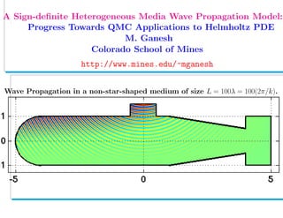
1. .
A Sign-definite Heterogeneous Media Wave Propagation Model:
Progress Towards QMC Applications to Helmholtz PDE
M. Ganesh
Colorado School of Mines
http://www.mines.edu/~mganesh
Wave Propagation in a non-star-shaped medium of size L = 100λ = 100(2π/k).

2. A Sign-definite Heterogeneous Media Wave Propagation Model:
Progress Towards QMC Applications to Helmholtz PDE
M. Ganesh
Colorado School of Mines
http://www.mines.edu/~mganesh
Wave Propagation in a star-shaped geometry of diamater L = 100λ = 100(2π/k).

3. State-of-the-art:QMC for PDEs with random coefficients
• F. Kuo and D. Nuyens (2011+ work with: Dick, LeGia, Schwab, Sloan...)
Application of QMC to elliptic PDEs with random diffusion coefficients
– a survey of analysis and implementation, J. FoCM, 2016

4. State-of-the-art:QMC for PDEs with random coefficients
• F. Kuo and D. Nuyens (2011+ work with: Dick, LeGia, Schwab, Sloan...)
Application of QMC to elliptic PDEs with random diffusion coefficients
– a survey of analysis and implementation, J. FoCM, 2016
Diffusion Model (with a random coefficient and zero Dirichlet BC):
−div[a(x, y) u] = f(x), x ∈ D ⊂ Rd
, for d = 2, 3, y ∈ U := [−1
2, 1
2]N
,
u(x, y) = 0, x ∈ ∂D, y ∈ U
Diffusion coefficient a(x, y) has an infinite parameter KL-type ansatz:
a(x, y) := a0(x) +
j≥1
aj(x, y) := a0(x) +
j≥1
yj ψj(x) , x ∈ D , y ∈ U

5. State-of-the-art:QMC for PDEs with random coefficients
• F. Kuo and D. Nuyens (2011+ work with: Dick, LeGia, Schwab, Sloan...)
Application of QMC to elliptic PDEs with random diffusion coefficients
– a survey of analysis and implementation, J. FoCM, 2016
Diffusion Model (with a random coefficient and zero Dirichlet BC):
−div[a(x, y) u] = f(x), x ∈ D ⊂ Rd
, for d = 2, 3, y ∈ U := [−1
2, 1
2]N
,
u(x, y) = 0, x ∈ ∂D, y ∈ U
Diffusion coefficient a(x, y) has an infinite parameter KL-type ansatz:
a(x, y) := a0(x) +
j≥1
aj(x, y) := a0(x) +
j≥1
yj ψj(x) , x ∈ D , y ∈ U
There exist amin, amax (that play crucial roles in POD/SPOD weights):
0 < amin ≤ a(x, y) ≤ amax < ∞, for all x ∈ D, y ∈ U
Hence, for each fixed y ∈ U, we obtain well-posedness in H1
0(Ω)
ψj: may belong to the KL eigensystem of a covariance operator

6. State-of-the-art:QMC for PDEs with random coefficients
• F. Kuo and D. Nuyens (2011+ work with: Dick, LeGia, Schwab, Sloan...)
Application of QMC to elliptic PDEs with random diffusion coefficients
– a survey of analysis and implementation, J. FoCM, 2016
Diffusion Model (with a random coefficient and zero Dirichlet BC):
−div[a(x, y) u] = f(x), x ∈ D ⊂ Rd
, for d = 2, 3, y ∈ U := [−1
2, 1
2]N
,
u(x, y) = 0, x ∈ ∂D, y ∈ U
Diffusion coefficient a(x, y) has an infinite parameter KL-type ansatz:
a(x, y) := a0(x) +
j≥1
aj(x, y) := a0(x) +
j≥1
yj ψj(x) , x ∈ D , y ∈ U
There exist amin, amax (that play crucial roles in POD/SPOD weights):
0 < amin ≤ a(x, y) ≤ amax < ∞, for all x ∈ D, y ∈ U
Hence, for each fixed y ∈ U, we obtain well-posedness in H1
0(Ω)
ψj: may belong to the KL eigensystem of a covariance operator
• 2014+: General operator form (Dick, LeGia, Kuo, Nuyens, Schwab):
La
u(x, y) :=

La0 + Laj

 u(x, y) = f(x), x ∈ D, y ∈ U,

7. Operator theory based diffusion model in heterogeneous media
• The general operator form allows for a large class of linear PDEs:

8. Operator theory based diffusion model in heterogeneous media
• The general operator form allows for a large class of linear PDEs:
For the strongly elliptic diffusion model with the KL-type ansatz:
La0v := −div[a0(x) v], Lajv := −yj div[ψj(x) v],
j≥1
ψj W1,∞ < ∞

9. Operator theory based diffusion model in heterogeneous media
• The general operator form allows for a large class of linear PDEs:
For the strongly elliptic diffusion model with the KL-type ansatz:
La0v := −div[a0(x) v], Lajv := −yj div[ψj(x) v],
j≥1
ψj W1,∞ < ∞
A standard bilinear form b0 : V × V → R for La0 with the mean-field
coefficient a0 > amin
0 (> 0) on D and V = H1
0(D) is sign-definite (coercive)
b0(v, v) := a0 v, v L2(D) :=
D
a0 | v|2
≥ Ccoer(amin
0 ) v 2
V > 0, v ∈ H1
0(D)

10. Operator theory based diffusion model in heterogeneous media
• The general operator form allows for a large class of linear PDEs:
For the strongly elliptic diffusion model with the KL-type ansatz:
La0v := −div[a0(x) v], Lajv := −yj div[ψj(x) v],
j≥1
ψj W1,∞ < ∞
A standard bilinear form b0 : V × V → R for La0 with the mean-field
coefficient a0 > amin
0 (> 0) on D and V = H1
0(D) is sign-definite (coercive)
b0(v, v) := a0 v, v L2(D) :=
D
a0 | v|2
≥ Ccoer(amin
0 ) v 2
V > 0, v ∈ H1
0(D)
Hence, in weak sense, we obtain invertibility of the strongly elliptic
operator La0 and its operator norm [La0]−1
depends on Ccoer
Ccoer plays a crucial role in POD/SPOD weights QMC constructions

11. Operator theory based diffusion model in heterogeneous media
• The general operator form allows for a large class of linear PDEs:
For the strongly elliptic diffusion model with the KL-type ansatz:
La0v := −div[a0(x) v], Lajv := −yj div[ψj(x) v],
j≥1
ψj W1,∞ < ∞
A standard bilinear form b0 : V × V → R for La0 with the mean-field
coefficient a0 > amin
0 (> 0) on D and V = H1
0(D) is sign-definite (coercive)
b0(v, v) := a0 v, v L2(D) :=
D
a0 | v|2
≥ Ccoer(amin
0 ) v 2
V > 0, v ∈ H1
0(D)
Hence, in weak sense, we obtain invertibility of the strongly elliptic
operator La0 and its operator norm [La0]−1
depends on Ccoer
Ccoer plays a crucial role in POD/SPOD weights QMC constructions
State-of-the-art in the general operator theoretic framework for well-
posedness of the model and QMC is to impose the assumption:
(Dick et al., SIAM J Numer. Anal., 2014, 2016 + ...., )
j≥1
[La0]−1
Laj
X→X
< 2

12. Operator theory based diffusion model in heterogeneous media
• The general operator form allows for a large class of linear PDEs:
For the strongly elliptic diffusion model with the KL-type ansatz:
La0v := −div[a0(x) v], Lajv := −yj div[ψj(x) v],
j≥1
ψj W1,∞ < ∞
A standard bilinear form b0 : V × V → R for La0 with the mean-field
coefficient a0 > amin
0 (> 0) on D and V = H1
0(D) is sign-definite (coercive)
b0(v, v) := a0 v, v L2(D) :=
D
a0 | v|2
≥ Ccoer(amin
0 ) v 2
V > 0, v ∈ H1
0(D)
Hence, in weak sense, we obtain invertibility of the strongly elliptic
operator La0 and its operator norm [La0]−1
depends on Ccoer
Ccoer plays a crucial role in POD/SPOD weights QMC constructions
State-of-the-art in the general operator theoretic framework for well-
posedness of the model and QMC is to impose the assumption:
(Dick et al., SIAM J Numer. Anal., 2014, 2016 + ...., )
j≥1
[La0]−1
Laj
X→X
< 2

13. Stochastic wave propagation model in heterogeneous media
• The general operator theory based assumption
j≥1
[La0]−1
Laj
X→X
< 2

14. Stochastic wave propagation model in heterogeneous media
• The general operator theory based assumption
j≥1
[La0]−1
Laj
X→X
< 2
facilities applicability to even a stochastic PDE model with all published
bilinear/sesquilinear forms of La0 that are NOT sign-definite

15. Stochastic wave propagation model in heterogeneous media
• The general operator theory based assumption
j≥1
[La0]−1
Laj
X→X
< 2
facilities applicability to even a stochastic PDE model with all published
bilinear/sesquilinear forms of La0 that are NOT sign-definite
• The sign-indefiniteness in sesquilinear forms can be tackled through the
alternative inf-suf framework. (Used also in QMC papers by Dick et al.,
SIAM J Numer. Anal., 2014, 2016 – a diffusion numerical example)

16. Stochastic wave propagation model in heterogeneous media
• The general operator theory based assumption
j≥1
[La0]−1
Laj
X→X
< 2
facilities applicability to even a stochastic PDE model with all published
bilinear/sesquilinear forms of La0 that are NOT sign-definite
• The sign-indefiniteness in sesquilinear forms can be tackled through the
alternative inf-suf framework. (Used also in QMC papers by Dick et al.,
SIAM J Numer. Anal., 2014, 2016 – a diffusion numerical example)
• Example (frequency-domain wave model): The standard sesquilinear form
in V = H1
(D) for the Helmholtz operator is not coercive (sign-indefinite)

17. Stochastic wave propagation model in heterogeneous media
• The general operator theory based assumption
j≥1
[La0]−1
Laj
X→X
< 2
facilities applicability to even a stochastic PDE model with all published
bilinear/sesquilinear forms of La0 that are NOT sign-definite
• The sign-indefiniteness in sesquilinear forms can be tackled through the
alternative inf-suf framework. (Used also in QMC papers by Dick et al.,
SIAM J Numer. Anal., 2014, 2016 – a diffusion numerical example)
• Example (frequency-domain wave model): The standard sesquilinear form
in V = H1
(D) for the Helmholtz operator is not coercive (sign-indefinite)
• The stochastic Helmholtz PDE model (with wavenumber k) can also be
written in the general operator form:
La0
k v = ∆v + k2
a0v, (L
aj
k v) = k2
yj ψjv, yj ∈ [−1
2, 1
2].
• The stochastic Helmholtz wave propagation model is:
−

La0
k +
j≥1
L
aj
k

 u(x, y) = f(x), x ∈ D, y ∈ U, + Absorbing BC on ∂D

18. Application of the general framework: Wavenumber restriction
• For establishing the well-posedness of the stochastic system, for each
y ∈ U, using the general framework, we need to verify the condition
j≥1
[La0]−1
k L
aj
k X→X
< 2

19. Application of the general framework: Wavenumber restriction
• For establishing the well-posedness of the stochastic system, for each
y ∈ U, using the general framework, we need to verify the condition
j≥1
[La0]−1
k L
aj
k X→X
< 2 (0.1)
• Establishing wavenumber-explicit bounds for [La0]−1
is still an open
problem for wave-trapping media with a heterogeneous wave propagation
domain D of interest [quantified by a refractive index a = cext/cD(ω), where
cext, cD are respectively the speed sound/light in the exterior and in D]

20. Application of the general framework: Wavenumber restriction
• For establishing the well-posedness of the stochastic system, for each
y ∈ U, using the general framework, we need to verify the condition
j≥1
[La0]−1
k L
aj
k X→X
< 2 (0.1)
• Establishing wavenumber-explicit bounds for [La0]−1
is still an open
problem for wave-trapping media with a heterogeneous wave propagation
domain D of interest [quantified by a refractive index a = cext/cD(ω), where
cext, cD are respectively the speed sound/light in the exterior and in D]
• For non-trapping media with D (say, star-shaped) the quantity
[La0]−1
depends linearly on k (Baskin..., SIAM J. Math. Anal., 2016)
• [Laj]v = k2
yj ψj v depends quadratically on the wavenumber k
• Hence even to establish well-posedness, the condition (0.1) requires
O(k3
) j≥1 .... < 2 , a severe restriction for practical cases k > 1

21. Application of the general framework: Wavenumber restriction
• For establishing the well-posedness of the stochastic system, for each
y ∈ U, using the general framework, we need to verify the condition
j≥1
[La0]−1
k L
aj
k X→X
< 2 (0.1)
• Establishing wavenumber-explicit bounds for [La0]−1
is still an open
problem for wave-trapping media with a heterogeneous wave propagation
domain D of interest [quantified by a refractive index a = cext/cD(ω), where
cext, cD are respectively the speed sound/light in the exterior and in D]
• For non-trapping media with D (say, star-shaped) the quantity
[La0]−1
depends linearly on k (Baskin..., SIAM J. Math. Anal., 2016)
• [Laj]v = k2
yj ψj v depends quadratically on the wavenumber k
• Hence even to establish well-posedness, the condition (0.1) requires
O(k3
) j≥1 .... < 2 , a severe restriction for practical cases k > 1
• Task: Avoid this restriction. Work on the PDE side or on the QMC side?
• Approach: A breakthrough Helmholtz PDE variational formulation and
a non-standard QMC analysis (WG for QMC part: Ganesh, Kuo, Sloan)

22. Stochastic wave propagation in random heterogeneous media
• Consider non-trapping wave propagation in Rd
, for d = 2, 3, comprising a
heterogeneous Lipschitz medium D with absorbing boundary ∂D
• The medium is described through a random and spatially variable index
of refraction a, modeled by the KL-type ansatz

23. Stochastic wave propagation in random heterogeneous media
• Consider non-trapping wave propagation in Rd
, for d = 2, 3, comprising a
heterogeneous Lipschitz medium D with absorbing boundary ∂D
• The medium is described through a random and spatially variable index
of refraction a, modeled by the KL-type ansatz
• Data: a forcing function f ∈ L2
(D) and boundary function gk ∈ L2
(∂D)
induced by an impinging incident wave (with wavenumber k)
• Randomness: for almost all events ω in the probability space (Ω, A, P),
• Find: an unknown stochastic wave-field u(·, ω) ∈ H1
(D) governed by the
Helmholtz PDE and an absorbing boundary condition:
∆u + k2
a(x, ω)u = −f(x), x ∈ Ω, ω ∈ (Ω, A, P)
∂u
∂ν
(x, ω) − iku(x, ω) = gk(x), x ∈ ∂Ω, ω ∈ (Ω, A, P)

24. Stochastic wave propagation in random heterogeneous media
• Consider non-trapping wave propagation in Rd
, for d = 2, 3, comprising a
heterogeneous Lipschitz medium D with absorbing boundary ∂D
• The medium is described through a random and spatially variable index
of refraction a, modeled by the KL-type ansatz
• Data: a forcing function f ∈ L2
(D) and boundary function gk ∈ L2
(∂D)
induced by an impinging incident wave (with wavenumber k)
• Randomness: for almost all events ω in the probability space (Ω, A, P),
• Find: an unknown stochastic wave-field u(·, ω) ∈ H1
(D) governed by the
Helmholtz PDE and an absorbing boundary condition:
∆u + k2
a(x, ω)u = −f(x), x ∈ Ω, ω ∈ (Ω, A, P)
∂u
∂ν
(x, ω) − iku(x, ω) = gk(x), x ∈ ∂Ω, ω ∈ (Ω, A, P)
• The random coefficient a(x, ω) is parameterized by a vector
y(ω) = (y1(ω), y2(ω), . . .)
.
• For a fixed realization y∗
, with a∗
(x) = a(x, y∗
) consider deterministic model

25. Deterministic wave propagation model in heterogeneous media
∆u(x) + k2
a∗
(x)u(x) = −f(x), x ∈ D
∂u
∂ν
(x) − iku(x) = g(x), x ∈ ∂D
• ν – outward unit normal; Data: f ∈ L2
(D), and g ∈ L2
(∂D)
• 0 < a∗
min ≤ a∗
(x) ≤ a∗
max < ∞, for all x ∈ D
• Literature: There exists a unique solution u ∈ H1
(D)

26. Deterministic wave propagation model in heterogeneous media
∆u(x) + k2
a∗
(x)u(x) = −f(x), x ∈ D
∂u
∂ν
(x) − iku(x) = g(x), x ∈ ∂D
• ν – outward unit normal; Data: f ∈ L2
(D), and g ∈ L2
(∂D)
• 0 < a∗
min ≤ a∗
(x) ≤ a∗
max < ∞, for all x ∈ D
• Literature: There exists a unique solution u ∈ H1
(D)
• Non-trapping media (A weaker non-trapping condition is sufficient.)

27. Deterministic wave propagation model in heterogeneous media
∆u(x) + k2
a∗
(x)u(x) = −f(x), x ∈ D
∂u
∂ν
(x) − iku(x) = g(x), x ∈ ∂D
• ν – outward unit normal; Data: f ∈ L2
(D), and g ∈ L2
(∂D)
• 0 < a∗
min ≤ a∗
(x) ≤ a∗
max < ∞, for all x ∈ D
• Literature: There exists a unique solution u ∈ H1
(D)
• Non-trapping media (A weaker non-trapping condition is sufficient.)
Figure 1: Example star-shaped domain D with refractive index a∗
∈ C1
(D) [but a∗
/∈ C2
(D)], with a∗
min = 1, a∗
max = 2

28. Standard Sign-Indefinite Variational Formulation

29. Standard Sign-Indefinite Variational Formulation
• Standard trial and test space: V = H1
(D)

30. Standard Sign-Indefinite Variational Formulation
• Standard trial and test space: V = H1
(D)
• Multiply by any test function v ∈ V and integrate:
- D(∆u + k2
a∗
u)v d x = D f(x)v d x

31. Standard Sign-Indefinite Variational Formulation
• Standard trial and test space: V = H1
(D)
• Multiply by any test function v ∈ V and integrate:
- D(∆u + k2
a∗
u)v d x = D f(x)v d x
• Apply the absorbing boundary condition to get the variational form:
• Solve: b(u, v) = F(v), for all v ∈ V,
b(u, v) = u, v L2(D) − k2
a∗
u, v L2(Ω) − ik u, v L2(∂D),
F(v) = f, v L2(D) + g, v L2(∂D).

32. Standard Sign-Indefinite Variational Formulation
• Standard trial and test space: V = H1
(D)
• Multiply by any test function v ∈ V and integrate:
- D(∆u + k2
a∗
u)v d x = D f(x)v d x
• Apply the absorbing boundary condition to get the variational form:
• Solve: b(u, v) = F(v), for all v ∈ V,
b(u, v) = u, v L2(D) − k2
a∗
u, v L2(Ω) − ik u, v L2(∂D),
F(v) = f, v L2(D) + g, v L2(∂D).
• The standard formulation is sign-indefinite (for sufficiently large k):
b(v, v) = v, v L2(D) − k2
a∗
v, v L2(D) < 0, v ∈ V

33. Standard Sign-Indefinite Variational Formulation
• Standard trial and test space: V = H1
(D)
• Multiply by any test function v ∈ V and integrate:
- D(∆u + k2
a∗
u)v d x = D f(x)v d x
• Apply the absorbing boundary condition to get the variational form:
• Solve: b(u, v) = F(v), for all v ∈ V,
b(u, v) = u, v L2(D) − k2
a∗
u, v L2(Ω) − ik u, v L2(∂D),
F(v) = f, v L2(D) + g, v L2(∂D).
• The standard formulation is sign-indefinite (for sufficiently large k):
b(v, v) = v, v L2(D) − k2
a∗
v, v L2(D) < 0, v ∈ V
• Because of the above, the Helmholtz PDE was (mis-)termed in many
publications as sign-indefinite and was (almost) accepted in the literature,
until a recent breakthrough was achieved

34. Is the Helmholtz equation really sign-indefinite?
• The above question and the resulting practical issues were considered
recently, for the homogeneous media [with n(x) = 1, x ∈ Ω] Helmholtz
PDE in two SIAM articles:
A. Moiola and E. Spence, SIAM Review, 2014
M. Ganesh and C. Morgenstern, SIAM J. Sci. Comput., 2017

35. Is the Helmholtz equation really sign-indefinite?
• The above question and the resulting practical issues were considered
recently, for the homogeneous media [with n(x) = 1, x ∈ Ω] Helmholtz
PDE in two SIAM articles:
A. Moiola and E. Spence, SIAM Review, 2014
M. Ganesh and C. Morgenstern, SIAM J. Sci. Comput., 2017
• Answer: The homogeneous Helmholtz model is NOT sign-indefinite.
That is,
(i) a natural Helmholtz PDE function space V ⊂ H1
(Ω) and a continuous
sesquilinear form b : V × V → C can be constructed with the property
that b(v, v) ≥ Ccoer v 2
V for all v ∈ V . [Proof with D is star-shaped.]
(ii) any solution u ∈ H1
(Ω) of the Helmholtz model satisfies the associ-
ated coercive variational (weak) formulation of the form
b(u, v) = G(v), for all v ∈ V
• Natural function space for the model with a solution u ∈ H1
(Ω) satisfying
∆u+k2
u = −f in Ω and ∂u
∂ν −iku = gk on ∂Ω, with data f ∈ L2
(Ω), gk ∈ L2
(∂Ω):
V := {v : v ∈ H1
(D), ∆v ∈ L2
(D), v ∈ H1
(∂D),
∂v
∂ν
∈ L2
(∂D)} ⊂ H3/2
(D)

36. Is the heterogeneous Helmholtz model really sign-indefinite?

37. Is the heterogeneous Helmholtz model really sign-indefinite?
• Answer with
a construtive continuous variational formulation and consistency anal-
ysis
wavenumber explicit bounds on the coercivity constant Ccoer (needed
for QMC weights, construction, weighted spaces and QMC-FEM )
a practical discrete high-order FEM formulation, a frequency robust
preconditioned FEM, and demonstrate using (parallel) implementation

38. Is the heterogeneous Helmholtz model really sign-indefinite?
• Answer with
a construtive continuous variational formulation and consistency anal-
ysis
wavenumber explicit bounds on the coercivity constant Ccoer (needed
for QMC weights, construction, weighted spaces and QMC-FEM )
a practical discrete high-order FEM formulation, a frequency robust
preconditioned FEM, and demonstrate using (parallel) implementation

39. Is the heterogeneous Helmholtz model really sign-indefinite?
• Answer with
a construtive continuous variational formulation and consistency anal-
ysis
wavenumber explicit bounds on the coercivity constant Ccoer (needed
for QMC weights, construction, weighted spaces and QMC-FEM )
a practical discrete high-order FEM formulation, a frequency robust
preconditioned FEM, and demonstrate using (parallel) implementation
• Done: M. Ganesh and C. Morgenstern, August 2017, Submitted
• The heterogeneous Helmholtz model is NOT sign-indefinite
• The coercivity constant Ccoer for the new sign-definite formulation is in-
dependent of the wavenumber (proved for star-shaped D)
• A high-order FEM with a non-standard preconditioner was developed
• A frequency-robust preconditioned FEM was constructed and implemented
for the sign-definite model
• Parallel implementation/demonstration includes hundreds of wavelengths
geometry D with curved and non-smooth Lipschitz boundaries

40. High-order FEM Sign-definite Approximations and Examples
• Choose a FEM space Vh ⊂ H2
(Ω) spanned by splines of degree p ≥ 2 on a
tessellation (with maximum width h) of Ω.
• Vh is chosen so that the following approximation property holds: For
v ∈ Hs0(Ω), with s0 ≥ 3/2, s = 0, 1, 2 and s < s0,
inf
wh∈Vh
||v − wh||Hs = O(hmin{p+1,s0}−s
)

41. High-order FEM Sign-definite Approximations and Examples
• Choose a FEM space Vh ⊂ H2
(Ω) spanned by splines of degree p ≥ 2 on a
tessellation (with maximum width h) of Ω.
• Vh is chosen so that the following approximation property holds: For
v ∈ Hs0(Ω), with s0 ≥ 3/2, s = 0, 1, 2 and s < s0,
inf
wh∈Vh
||v − wh||Hs = O(hmin{p+1,s0}−s
)
• We simulate low to high-frequency ( 1 to 400 wavelengths problems) with
and without a novel frequency-robust preconditioner for a star-shaped
(below) and a non-star shaped geometry using a spatially variable refrac-
tive index a∗
∈ C1
(D), but a∗
/∈ C2
(D)

42. FEM Accuracy Verifications: Smooth & Non-smooth solutions
• Two test cases (with uh simulated using high-order FEMs with p ≥ 2) :
Smooth exact (wavenumber dependent) solution:
u = u∗,k
∈ Hs0(Ω), for all s0 ≥ 2.
Expected optimal order convergence:
||u∗,k
− uh||Hs(Ω) = O(hp+1−s
), s = 0, 1, 2

43. FEM Accuracy Verifications: Smooth & Non-smooth solutions
• Two test cases (with uh simulated using high-order FEMs with p ≥ 2) :
Smooth exact (wavenumber dependent) solution:
u = u∗,k
∈ Hs0(Ω), for all s0 ≥ 2.
Expected optimal order convergence:
||u∗,k
− uh||Hs(Ω) = O(hp+1−s
), s = 0, 1, 2
Non-smooth exact solution u = u†,k
∈ Hs0(Ω) for s0 with 3/2 ≤ s0 < 2:
Expected optimal order convergence ||u†,k
− uh||Hs(Ω) = O(hs0−s
), s = 0, 1

44. FEM Accuracy Verifications: Smooth & Non-smooth solutions
• Two test cases (with uh simulated using high-order FEMs with p ≥ 2) :
Smooth exact (wavenumber dependent) solution:
u = u∗,k
∈ Hs0(Ω), for all s0 ≥ 2.
Expected optimal order convergence:
||u∗,k
− uh||Hs(Ω) = O(hp+1−s
), s = 0, 1, 2
Non-smooth exact solution u = u†,k
∈ Hs0(Ω) for s0 with 3/2 ≤ s0 < 2:
Expected optimal order convergence ||u†,k
− uh||Hs(Ω) = O(hs0−s
), s = 0, 1
• Smooth exact point-source solution, with source centered at x∗
= (0, 3) :
The input source and boundary functions f and g of the wave propagation
model are chosen so that the exact solution is given by
u∗,k
(x) = Gk(x, x∗
) =
i
4
H
(1)
0 (k| x −x∗
|),
where H
(1)
0 denotes the Hankel function of the first kind of order zero.

45. Sign-definite FEM Optimal O(hp+1−s) Verifications: Smooth
p=2, L = 5λ
h L2
Error EOC H1
Error EOC H2
Error EOC V Error EOC
(1/2)3
9.8632e-05 – 1.9547e-03 – 6.0705e-02 – 1.1927e-02 –
(1/2)4
1.1731e-05 3.07 4.8131e-04 2.02 3.0265e-02 1.00 5.8430e-03 1.03
(1/2)5
1.4813e-06 2.99 1.1980e-04 2.01 1.5117e-02 1.00 2.9093e-03 1.01
(1/2)6
1.8907e-07 2.97 2.9862e-05 2.00 7.5557e-03 1.00 1.4538e-03 1.00
p=3, L = 5λ

46. Sign-definite FEM Optimal O(hp+1−s) Verifications: Smooth
p=2, L = 5λ
h L2
Error EOC H1
Error EOC H2
Error EOC V Error EOC
(1/2)3
9.8632e-05 – 1.9547e-03 – 6.0705e-02 – 1.1927e-02 –
(1/2)4
1.1731e-05 3.07 4.8131e-04 2.02 3.0265e-02 1.00 5.8430e-03 1.03
(1/2)5
1.4813e-06 2.99 1.1980e-04 2.01 1.5117e-02 1.00 2.9093e-03 1.01
(1/2)6
1.8907e-07 2.97 2.9862e-05 2.00 7.5557e-03 1.00 1.4538e-03 1.00
p=3, L = 5λ
h L2
Error EOC H1
Error EOC H2
Error EOC V Error EOC
(1/2)3
3.9910e-06 – 7.6141e-05 – 2.0158e-03 – 3.9456e-04 –
(1/2)4
2.3445e-07 4.09 9.3670e-06 3.02 4.9631e-04 2.02 9.5597e-05 2.05
(1/2)5
1.5200e-08 3.95 1.1692e-06 3.00 1.2337e-04 2.01 2.3716e-05 2.01
(1/2)6
9.4110e-10 4.01 1.4548e-07 3.01 3.0793e-05 2.00 5.9228e-06 2.00
p=4, L = 5λ

47. Sign-definite FEM Optimal O(hp+1−s) Verifications: Smooth
p=2, L = 5λ
h L2
Error EOC H1
Error EOC H2
Error EOC V Error EOC
(1/2)3
9.8632e-05 – 1.9547e-03 – 6.0705e-02 – 1.1927e-02 –
(1/2)4
1.1731e-05 3.07 4.8131e-04 2.02 3.0265e-02 1.00 5.8430e-03 1.03
(1/2)5
1.4813e-06 2.99 1.1980e-04 2.01 1.5117e-02 1.00 2.9093e-03 1.01
(1/2)6
1.8907e-07 2.97 2.9862e-05 2.00 7.5557e-03 1.00 1.4538e-03 1.00
p=3, L = 5λ
h L2
Error EOC H1
Error EOC H2
Error EOC V Error EOC
(1/2)3
3.9910e-06 – 7.6141e-05 – 2.0158e-03 – 3.9456e-04 –
(1/2)4
2.3445e-07 4.09 9.3670e-06 3.02 4.9631e-04 2.02 9.5597e-05 2.05
(1/2)5
1.5200e-08 3.95 1.1692e-06 3.00 1.2337e-04 2.01 2.3716e-05 2.01
(1/2)6
9.4110e-10 4.01 1.4548e-07 3.01 3.0793e-05 2.00 5.9228e-06 2.00
p=4, L = 5λ
h L2
Error EOC H1
Error EOC H2
Error EOC V Error EOC
(1/2)3
1.7368e-07 – 3.1041e-06 – 7.9122e-05 – 1.5297e-05 –
(1/2)4
5.1704e-09 5.07 1.8832e-07 4.04 9.7815e-06 3.02 1.8783e-06 3.03
(1/2)5
1.6033e-10 5.01 1.1627e-08 4.02 1.2201e-06 3.00 2.3448e-07 3.00
(1/2)6
4.7944e-12 5.06 7.2152e-10 4.01 1.5256e-07 3.00 2.9344e-08 3.00

48. Sign-definite FEM Optimal O(hs0−s) Verifications: Non-smooth
• Define a function that is NOT in H2
(Ω) and in Hs0(Ω) with 3/2 < s0 < 2:

49. Sign-definite FEM Optimal O(hs0−s) Verifications: Non-smooth
• Define a function that is NOT in H2
(Ω) and in Hs0(Ω) with 3/2 < s0 < 2:
u†,k
(x) = Cu∗,k
(x) m†
(q(x)) , m†
: [0, 1] × [0, 1] → R, with m†
(y) = y
3/2
1 y
3/2
2 ,
where for x = (x1, x2) ∈ Ω, let q : Ω → [0, 1] × [0, 1] with
q(x) = (−0.1x1 + 0.5, 0.5x2 + 0.5)

50. Sign-definite FEM Optimal O(hs0−s) Verifications: Non-smooth
• Define a function that is NOT in H2
(Ω) and in Hs0(Ω) with 3/2 < s0 < 2:
u†,k
(x) = Cu∗,k
(x) m†
(q(x)) , m†
: [0, 1] × [0, 1] → R, with m†
(y) = y
3/2
1 y
3/2
2 ,
where for x = (x1, x2) ∈ Ω, let q : Ω → [0, 1] × [0, 1] with
q(x) = (−0.1x1 + 0.5, 0.5x2 + 0.5)
p=3, L = 5λ
h L2
Error EOC H1
Error EOC
(1/2)4
1.7015e-05 – 3.8796e-04 –
(1/2)5
8.2279e-06 1.05 3.3090e-04 0.23
(1/2)6
2.6762e-06 1.62 1.9650e-04 0.75
(1/2)7
7.1197e-07 1.91 1.0321e-04 0.93
p=4, L = 5λ

51. Sign-definite FEM Optimal O(hs0−s) Verifications: Non-smooth
• Define a function that is NOT in H2
(Ω) and in Hs0(Ω) with 3/2 < s0 < 2:
u†,k
(x) = Cu∗,k
(x) m†
(q(x)) , m†
: [0, 1] × [0, 1] → R, with m†
(y) = y
3/2
1 y
3/2
2 ,
where for x = (x1, x2) ∈ Ω, let q : Ω → [0, 1] × [0, 1] with
q(x) = (−0.1x1 + 0.5, 0.5x2 + 0.5)
p=3, L = 5λ
h L2
Error EOC H1
Error EOC
(1/2)4
1.7015e-05 – 3.8796e-04 –
(1/2)5
8.2279e-06 1.05 3.3090e-04 0.23
(1/2)6
2.6762e-06 1.62 1.9650e-04 0.75
(1/2)7
7.1197e-07 1.91 1.0321e-04 0.93
p=4, L = 5λ
h L2
Error EOC H1
Error EOC
(1/2)4
1.3915e-05 – 3.8780e-04 –
(1/2)5
4.5897e-06 1.60 2.5599e-04 0.60
(1/2)6
1.2443e-06 1.88 1.3777e-04 0.89
(1/2)7
3.2821e-07 1.92 7.1168e-05 0.95

52. High-order FEM Accuracy for High-frequency Simulations
• L2
(Ω)-norm error for the non-smooth problem for various high-frequency
with h = (1/2)7
.
L 50λ 100λ 150λ 200λ
p=2 2.3630e-05 3.1956e-04 2.0659e-03 8.4938e-03
p=3 5.4271e-07 8.7587e-06 4.8182e-05 1.8524e-04
p=4 6.9149e-08 4.8657e-07 3.9483e-06 1.8401e-05

53. High-order FEM Accuracy for High-frequency Simulations
• L2
(Ω)-norm error for the non-smooth problem for various high-frequency
with h = (1/2)7
.
L 50λ 100λ 150λ 200λ
p=2 2.3630e-05 3.1956e-04 2.0659e-03 8.4938e-03
p=3 5.4271e-07 8.7587e-06 4.8182e-05 1.8524e-04
p=4 6.9149e-08 4.8657e-07 3.9483e-06 1.8401e-05
L 250λ 300λ 350λ 400λ
p=2 2.6176e-02 6.7126e-02 1.5155e-01 3.1067e-01
p=3 6.5186e-04 2.2050e-03 6.9045e-03 1.9635e-02
p=4 6.3918e-05 1.9098e-04 5.5490e-04 1.7007e-03

54. A New Class of Frequency-robust Preconditioned FEM
• Consider the complex-shifted heterogeneous model with
Ln
Eu(x) = ∆u + (k2
+ i E)nu

55. A New Class of Frequency-robust Preconditioned FEM
• Consider the complex-shifted heterogeneous model with
Ln
Eu(x) = ∆u + (k2
+ i E)nu
Ln
EuE = −f, x ∈ Ω
∂uE
∂ν
− ikuE = g, x ∈ ∂Ω
We derive an associated preconditioner sesquilinear form using Ln
E and
Ln
Eu = ∆u + (k2
+ i E)nu

56. A New Class of Frequency-robust Preconditioned FEM
• Consider the complex-shifted heterogeneous model with
Ln
Eu(x) = ∆u + (k2
+ i E)nu
Ln
EuE = −f, x ∈ Ω
∂uE
∂ν
− ikuE = g, x ∈ ∂Ω
We derive an associated preconditioner sesquilinear form using Ln
E and
Ln
Eu = ∆u + (k2
+ i E)nu

57. Simulation: Frequency-Independent Precond. FEM Iterations
• Inner iterations required for GMRES(10) with p = 4, h = (1/2)7
, β = 106
E = (1/4)k E = (1/2)k Unprecondtioned
L ITER Time (s) ITER Time (s) ITER Time (s)
50λ 7 312.87 10 386.72 128869 17707.40
100λ 7 284.21 10 387.07 195248 26761.17
150λ 7 282.41 10 432.61 223566 28885.00
200λ 7 283.51 10 388.21 225474 28856.81
250λ 7 309.11 10 385.99 223326 30615.33
300λ 7 283.07 10 432.32 227209 31097.47
350λ 7 285.89 10 390.28 264440 34033.65
400λ 7 281.86 10 391.07 304191 39235.95

58. Simulation: Validation for a Non-star-shaped Geometry
• We use the parameters chosen for a similar star-shaped geometry for the
following non-star-shaped geometry:
Figure 3: The example geometry and refractive index n(x).

59. Non-star-shaped – FEM Optimal O(hp+1−s) Verifications: Smoo
p=2, L = 5λ
h L2
Error EOC H1
Error EOC H2
Error EOC V Error EOC
(1/2)3
1.0376e-04 3.27 1.9819e-03 2.09 6.0883e-02 1.02 1.1706e-02 1.17
(1/2)4
1.1990e-05 3.11 4.8389e-04 2.03 3.0298e-02 1.01 5.6591e-03 1.05
(1/2)5
1.5007e-06 3.00 1.2014e-04 2.01 1.5125e-02 1.00 2.8055e-03 1.01
(1/2)6
1.9029e-07 2.98 2.9901e-05 2.01 7.5575e-03 1.00 1.3993e-03 1.00
p=3, L = 5λ
h L2
Error EOC H1
Error EOC H2
Error EOC V Error EOC
(1/2)3
4.1249e-06 4.31 7.8331e-05 3.15 2.0613e-03 2.11 4.0120e-04 2.31
(1/2)4
2.3780e-07 4.12 9.4643e-06 3.05 5.0039e-04 2.04 9.3534e-05 2.10
(1/2)5
1.5322e-08 3.96 1.1747e-06 3.01 1.2378e-04 2.02 2.2943e-05 2.03
(1/2)6
9.4801e-10 4.01 1.4579e-07 3.01 3.0828e-05 2.01 5.7060e-06 2.01
p=4, L = 5λ
h L2
Error EOC H1
Error EOC H2
Error EOC V Error EOC
(1/2)3
1.8034e-07 5.31 3.2030e-06 4.22 8.4066e-05 3.19 1.6392e-05 3.41
(1/2)4
5.2717e-09 5.10 1.9023e-07 4.07 9.9774e-06 3.07 1.8616e-06 3.14
(1/2)5
1.6372e-10 5.01 1.1690e-08 4.02 1.2298e-06 3.02 2.2788e-07 3.03
(1/2)6
4.8773e-12 5.07 7.2331e-10 4.01 1.5293e-07 3.01 2.8305e-08 3.01

60. Non-star-shaped: Frequency-Independent PFEM Iterations
• Inner iterations required for GMRES(10) with p = 4, h = (1/2)7
, β = 106
E = (1/4)k E = (1/2)k Unprecondtioned
L ITER Time (s) ITER Time (s) ITER Time (s)
50λ 7 262.92 10 320.72 * *
100λ 7 262.93 10 362.77 * *
150λ 7 261.16 10 361.81 341014 43706.09
200λ 7 264.10 10 360.63 271793 34656.75
250λ 7 263.05 10 363.66 246396 31044.40
300λ 7 263.36 10 362.80 255680 33132.92
350λ 7 264.60 10 330.04 275385 35290.32
400λ 7 265.00 10 366.36 328849 42136.47