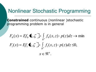
Download as PDF, PPTX


![Nonlinear Stochastic Programming
Procedure for stochastic optimization:
t 1 t ~
x x x L( x t , t
)
t 1 t ~ t ~
max[0, ( F1 ( x ) DF1 ( x t ))]
0 0 0
N , , x - initial values
- parameters of
0, 0 optimization](https://image.slidesharecdn.com/lecture4-100818114030-phpapp02/85/Nonlinear-Stochastic-Programming-by-the-Monte-Carlo-method-23-320.jpg)


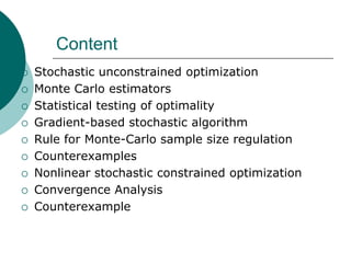
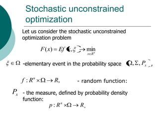
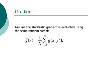
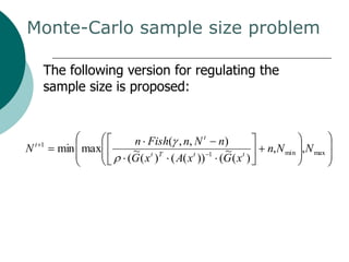
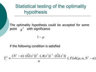
The document discusses nonlinear stochastic programming using the Monte Carlo method, covering aspects like stochastic unconstrained optimization, Monte Carlo estimators, and gradient-based algorithms. It presents a methodology for optimizing sample sizes and statistical testing of optimality in optimization problems, alongside specific applications such as manpower planning. The conclusions highlight the effectiveness of the proposed approach for reliable testing of optimality in a wide range of stochastic optimization scenarios.