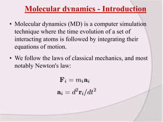
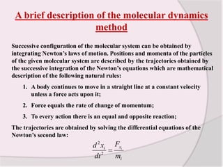
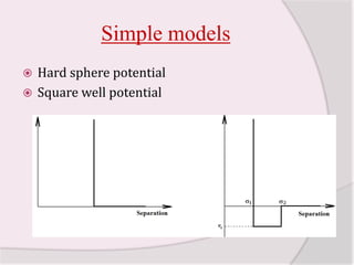
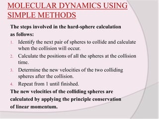
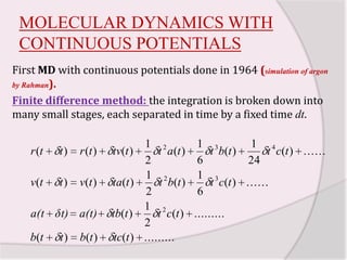
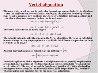
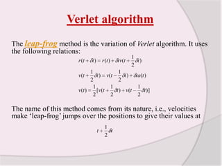
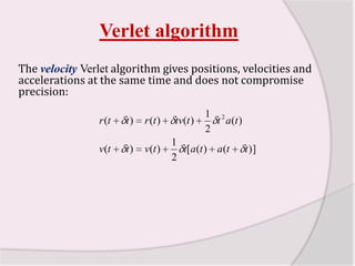
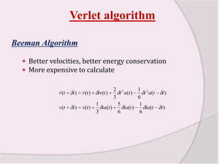
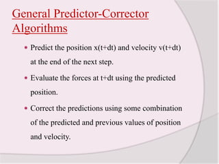
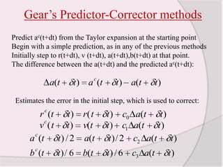
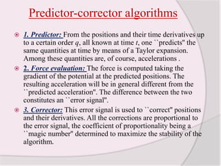
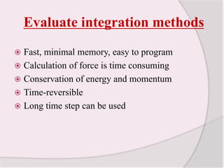
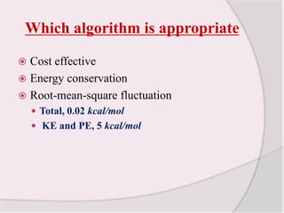
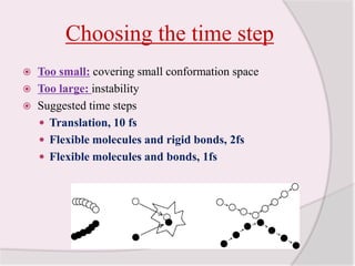
MOLECULAR DYNAMIC SIMULATION METHODS
Molecular dynamics - IntroductionMolecular dynamics (MD) is a computer simulation technique where the time evolution of a set of interacting atoms is followed by integrating their equations of motion.
We follow the laws of classical mechanics, and most notably Newton's law: A brief description of the molecular dynamics methodSuccessive configuration of the molecular system can be obtained by integrating Newton’s laws of motion. Positions and momenta of the particles of the given molecular system are described by the trajectories obtained by the successive integration of the Newton’s equations which are mathematical description of the following natural rules:A body continues to move in a straight line at a constant velocity unless a force acts upon it;Force equals the rate of change of momentum;To every action there is an equal and opposite reaction;The trajectories are obtained by solving the differential equations of the Newton’s second law:
Simple modelsHard sphere potentialSquare well potential
MOLECULAR DYNAMICS USING SIMPLE METHODSThe steps involved in the hard-sphere calculationas follows:Identify the next pair of spheres to collide and calculate when the collision will occur.Calculate the positions of all the spheres at the collision time.Determine the new velocities of the two colliding spheres after the collision.Repeat from 1 until finished.The new velocities of the colliding spheres are calculated by applying the principle conservationof linear momentum.
MOLECULAR DYNAMICS WITH CONTINUOUS POTENTIALSFirst MD with continuous potentials done in 1964 (simulation of argon by Rahman). Finite difference method: the integration is broken down into many small stages, each separated in time by a fixed time dt.
Verlet algorithmThe most widely used method in molecular dynamics programs is the Verlet algorithm. It uses the positions and accelerations at time t, and the positions from the previous step, r(t-δt) to calculate new positions at t+δt, r(t+δt). Relations between positions and velocities at those two moments in time can be written as:Those two relations can be added to give:The velocities do not explicitly appear in the Verlet algorithm. They can be calculated in several ways. A very simple approach is to divide the difference in positions at times t+δt and t-δt by 2δt, i.e. Another approach calculates velocities at the half step              :Practical application of this algorithm is straightforward and memory requirements are modest, only positions at two time steps have to be recorded r(t), r(t-δt), and the acceleration a(t). The only drawback is that the new position r(t + δt) is obtained by adding small term δ2ta(t) to the difference of two much larger terms 2r(t) and r(t-δt), which requires high precision for r in the numerical calculation.
Verlet algorithmThe leap-frog method is the variation of Verlet algorithm. It uses the following relations:The name of this method comes from its nature, i.e., velocities make ‘leap-frog’ jumps over the positions to give their values at
Verlet algorithmThe velocity Verlet algorithm gives positions, velocities and accelerations at the same time and does not compromise precision:
Verlet algorithmBeeman AlgorithmBetter velocities, better energy conservationMore expensive to calculate
General Predictor-Corrector AlgorithmsPredict the position x(t+dt) and velocity v(t+dt) at the end of the next step.Evaluate the forces at t+dt using the predicted position.Correct the predictions using some combination of the predicted and previous values of position and velocity.
Gear’s Predictor-Corrector methodsPredict ac(t+dt) from the Taylor expansion at the starting pointBegin with a simple prediction, as in any of the previous methodsInitially step to r(t+dt), v (t+dt), a(t+dt),b(t+dt) at that point.The difference between the a(t+dt) and the predicted ac(t+dt): Estimates the error in the initial step, which is used to correct:
Predictor-corrector algorithms1. Predictor: From the positions and their time derivatives up to a certain order q, all known at time t, one ``predicts'' the same quantities at time by means of a Taylor expansion. Among these quantities are, of course, accelerations .2. Force evaluation: The force is computed taking the gradient of the potential at the predicted positions. The resulting acceleration will be in general different from the ``predicted acceleration''. The difference between the two constitutes an ``error signal''. 3. Corrector: This error signal is used to ``correct'' positions and their derivatives. All the corrections are proportional to the error signal, the coefficient of proportionality being a ``magic number'' determined to maximize the stability of the algorithm.
Evaluate integration methodsFast, minimal memory, easy to programCalculation of force is time consumingConservation of energy and momentumTime-reversibleLong time step can be used
Which algorithm is appropriateCost effectiveEnergy conservationRoot-mean-square fluctuationTotal, 0.02 kcal/mol KE and PE, 5 kcal/mol
Choosing the time stepToo small: covering small conformation spaceToo large: instabilitySuggested time stepsTranslation, 10 fsFlexible molecules and rigid bonds, 2fsFlexible molecules and bonds, 1fs
Multiple time step dynamicsReversible reference system propagation algorithm (r-RESPA)Forces within a system classified into a number of groups according to how rapidly the force changesEach group has its own time step, while maintaining accuracy and numerical stability
Molecular dynamics setupInitial configurationInitial velocities (Maxwell-Boltzmann)Force fieldCutoff: doesn’t save time by itself. But can combine with neighbor list and speed-up the simulation
Running molecular dynamicsEquilibrationSpecial care is needed for inhomogeneous systemCalculating the temperatureNc is the number of constraints, so 3N – Nc is the total number of degrees of freedomBoundary conditionsNo boundaryPeriodic boundary conditionNon-periodic: reaction zone, harmonic constraint boundary atoms
Constraint dynamicsHigh frequency modes takes all the computer timeLow frequency modes correspond to conformational changesConstraint: system is forced to satisfy certain conditionsSHAKE: constraint the bond vibration
REFERENCEMolecular Modelling      -   Andrew R. Leach(Principles and Applications)http:/docjax.com/molecular dynamic simulation methods/http:/google.com/molecular dynamics/ simulation simple methods/http:/google.com/molecular dynamic simulation with continuous potential/
THANQ

MOLECULAR SIMULATION TECHNIQUES

  • 1.
  • 2.
    Molecular dynamics -IntroductionMolecular dynamics (MD) is a computer simulation technique where the time evolution of a set of interacting atoms is followed by integrating their equations of motion.
  • 3.
    We follow thelaws of classical mechanics, and most notably Newton's law: A brief description of the molecular dynamics methodSuccessive configuration of the molecular system can be obtained by integrating Newton’s laws of motion. Positions and momenta of the particles of the given molecular system are described by the trajectories obtained by the successive integration of the Newton’s equations which are mathematical description of the following natural rules:A body continues to move in a straight line at a constant velocity unless a force acts upon it;Force equals the rate of change of momentum;To every action there is an equal and opposite reaction;The trajectories are obtained by solving the differential equations of the Newton’s second law:
  • 4.
    Simple modelsHard spherepotentialSquare well potential
  • 5.
    MOLECULAR DYNAMICS USINGSIMPLE METHODSThe steps involved in the hard-sphere calculationas follows:Identify the next pair of spheres to collide and calculate when the collision will occur.Calculate the positions of all the spheres at the collision time.Determine the new velocities of the two colliding spheres after the collision.Repeat from 1 until finished.The new velocities of the colliding spheres are calculated by applying the principle conservationof linear momentum.
  • 6.
    MOLECULAR DYNAMICS WITHCONTINUOUS POTENTIALSFirst MD with continuous potentials done in 1964 (simulation of argon by Rahman). Finite difference method: the integration is broken down into many small stages, each separated in time by a fixed time dt.
  • 7.
    Verlet algorithmThe mostwidely used method in molecular dynamics programs is the Verlet algorithm. It uses the positions and accelerations at time t, and the positions from the previous step, r(t-δt) to calculate new positions at t+δt, r(t+δt). Relations between positions and velocities at those two moments in time can be written as:Those two relations can be added to give:The velocities do not explicitly appear in the Verlet algorithm. They can be calculated in several ways. A very simple approach is to divide the difference in positions at times t+δt and t-δt by 2δt, i.e. Another approach calculates velocities at the half step :Practical application of this algorithm is straightforward and memory requirements are modest, only positions at two time steps have to be recorded r(t), r(t-δt), and the acceleration a(t). The only drawback is that the new position r(t + δt) is obtained by adding small term δ2ta(t) to the difference of two much larger terms 2r(t) and r(t-δt), which requires high precision for r in the numerical calculation.
  • 8.
    Verlet algorithmThe leap-frogmethod is the variation of Verlet algorithm. It uses the following relations:The name of this method comes from its nature, i.e., velocities make ‘leap-frog’ jumps over the positions to give their values at
  • 9.
    Verlet algorithmThe velocityVerlet algorithm gives positions, velocities and accelerations at the same time and does not compromise precision:
  • 10.
    Verlet algorithmBeeman AlgorithmBettervelocities, better energy conservationMore expensive to calculate
  • 11.
    General Predictor-Corrector AlgorithmsPredictthe position x(t+dt) and velocity v(t+dt) at the end of the next step.Evaluate the forces at t+dt using the predicted position.Correct the predictions using some combination of the predicted and previous values of position and velocity.
  • 12.
    Gear’s Predictor-Corrector methodsPredictac(t+dt) from the Taylor expansion at the starting pointBegin with a simple prediction, as in any of the previous methodsInitially step to r(t+dt), v (t+dt), a(t+dt),b(t+dt) at that point.The difference between the a(t+dt) and the predicted ac(t+dt): Estimates the error in the initial step, which is used to correct:
  • 13.
    Predictor-corrector algorithms1. Predictor:From the positions and their time derivatives up to a certain order q, all known at time t, one ``predicts'' the same quantities at time by means of a Taylor expansion. Among these quantities are, of course, accelerations .2. Force evaluation: The force is computed taking the gradient of the potential at the predicted positions. The resulting acceleration will be in general different from the ``predicted acceleration''. The difference between the two constitutes an ``error signal''. 3. Corrector: This error signal is used to ``correct'' positions and their derivatives. All the corrections are proportional to the error signal, the coefficient of proportionality being a ``magic number'' determined to maximize the stability of the algorithm.
  • 14.
    Evaluate integration methodsFast,minimal memory, easy to programCalculation of force is time consumingConservation of energy and momentumTime-reversibleLong time step can be used
  • 15.
    Which algorithm isappropriateCost effectiveEnergy conservationRoot-mean-square fluctuationTotal, 0.02 kcal/mol KE and PE, 5 kcal/mol
  • 16.
    Choosing the timestepToo small: covering small conformation spaceToo large: instabilitySuggested time stepsTranslation, 10 fsFlexible molecules and rigid bonds, 2fsFlexible molecules and bonds, 1fs
  • 17.
    Multiple time stepdynamicsReversible reference system propagation algorithm (r-RESPA)Forces within a system classified into a number of groups according to how rapidly the force changesEach group has its own time step, while maintaining accuracy and numerical stability
  • 18.
    Molecular dynamics setupInitialconfigurationInitial velocities (Maxwell-Boltzmann)Force fieldCutoff: doesn’t save time by itself. But can combine with neighbor list and speed-up the simulation
  • 19.
    Running molecular dynamicsEquilibrationSpecialcare is needed for inhomogeneous systemCalculating the temperatureNc is the number of constraints, so 3N – Nc is the total number of degrees of freedomBoundary conditionsNo boundaryPeriodic boundary conditionNon-periodic: reaction zone, harmonic constraint boundary atoms
  • 20.
    Constraint dynamicsHigh frequencymodes takes all the computer timeLow frequency modes correspond to conformational changesConstraint: system is forced to satisfy certain conditionsSHAKE: constraint the bond vibration
  • 21.
    REFERENCEMolecular Modelling - Andrew R. Leach(Principles and Applications)http:/docjax.com/molecular dynamic simulation methods/http:/google.com/molecular dynamics/ simulation simple methods/http:/google.com/molecular dynamic simulation with continuous potential/
  • 22.