1) Molecular dynamics (MD) simulations numerically solve Newton's equations of motion to simulate the physical movements of atoms and molecules over time. 2) The Verlet algorithm is commonly used to integrate the equations of motion in MD simulations. It calculates new positions and velocities at each time step based on the forces between particles. 3) MD simulations sample the ensemble of all possible configurations over time. If run long enough, time averages from the simulation converge to ensemble averages, in accordance with the ergodic hypothesis. This allows MD to connect microscopic dynamics to macroscopic thermodynamics.

1. 1
Molecular Biophysics III – dynamics
Molecular Dynamics Simulations - 01/13/05
Hagai Meirovitch

2. 2
References:
1) A.R. Leach, “Molecular Modeling”, second edition, Prentice Hall
pp. 353-406.
2) D. Frenkel and B. Smit, “Understanding Molecular Simulations from
Algorithms to Applications”, second edition, Academic Press.
Chapters 4 and 6.
3) M.P. Allen and D. J. Tildesley, “Computer Simulation of Liquids”,
1991, Oxford. Chapter 3.

3. 3
Introduction
Biological processes are commonly studied by experimental techniques
(X-ray, NMR, etc.). However, to gain deeper insights in terms of atomic
interactions we try to model biological macromolecules (proteins, DNA,
carbohydrates, etc.) and simulate their behavior by Monte Carlo (MC)
methods or molecular dynamics (MD) techniques that obey the rules of
physics.
Before discussing MD let us refresh some basic notions from high school
physics.

4. 4
Forces
Examples of F (F vector; F=|F|) :
1) Stretching a spring by a distance x: F= -fx, Hook’s Law
f- spring constant. F negative because it is opposite to x.
2) Gravitation force: F= kMm/r2 - m and M masses with distance r; k -
constant. On earth (R,M large), g=kM/R2  F=mg
3) Coulomb law: F=kq1q2/r2 , q1 and q2 charges.
Newton’s second law (F - resultant force):
a, v, and x vectors; t time
2
2
dt
d
m
dt
d
m
m
x
v
a
F 



5. 5
Mechanical work W:
If a constant force is applied along distance d, W=Fd (F=|F|). More
general, W=! F.dx.
Potential energy:
If mass m is raised to height h negative work is done, W = –mgh and the
mass gains potential energy,Ep= -W = +mgh - the ability to do
mechanical work: when m falls dawn, Ep is converted into
kinetic energy,
Ek = mv2/2, where v2/2=gh (at floor).
A spring stretched by d: Ep= -W = f! xdx = fd2/2
Two charges: Ep = kq1q2/r
In a closed system the total energy, Etot = Ep+ Ek is constant but Ep/Ek can
change; e.g., oscillation of a mass hung on a spring.

6. 6
Linear momentum
p=mv
The total momentum of a system of particles is equal to the momentum
of a single particle with the total mass of the system moving with the
velocity of the center of mass of the system, vCM
vCM = Σmivi / Σmi
In a system with no external forces the total momentum is conserved -
the center of mass moves in a straight line with constant speed.
Notice, the force exerted on a particle is the negative derivative of the
potential energy with respect to the coordinates.
F = dp/dt = - dEp/dx

7. 7


















 



6
12
4
r
r
r)
(
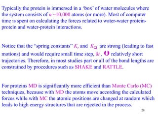
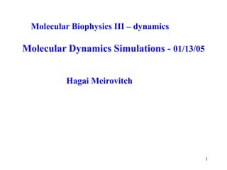
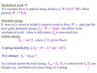
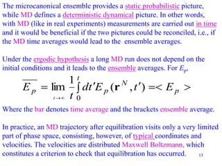
MD simulations
We treat N argon atoms of mass m enclosed in an isolated container.
Each pair interacts via Lennard-Jones potential energy (Etot= const.)
r =σ
ε
r
The force in x1 direction between (x1, y1, z1) and (x2, y2, z2)
r
x
r
r
r
x
r
x
z
z
y
y
x
x
r
x
r
r
x
Fx
1
7
6
13
12
1
1
2
/
1
2
2
1
2
2
1
2
2
1
1
1
2
24
]
)
(
)
(
)
[(
1





 



































8. 8
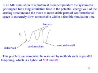
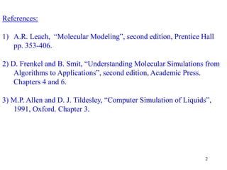
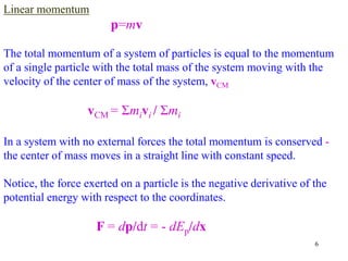
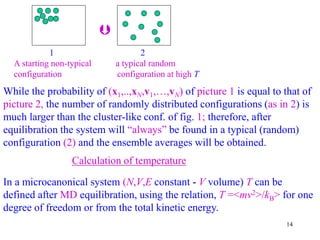
Assume that at t=0 atom i is positioned at coordinates xi(0) and has
initial velocity vi(0) (i=1,N); one can solve numerically Newton’s
equations obtaining the positions xi(t) and velocities vi(t) at time t. This
is the essence of MD.
Integration of the equations of motion by a finite differences method
with the popular Verlet algorithm: Taylor expansions to 3rd order for i
Adding these equations gives [up to order (δt)4]
Independent of velocities. a(t) is calculated from F/m; m – mass.
.....
)
(
)
(
6
1
)
(
)
(
2
1
)
(
)
(
)
(
)
(
....
)
(
)
(
6
1
)
(
)
(
2
1
)
(
)
(
)
(
)
(
3
2
3
2




















t
t
t
t
t
t
t
t
t
t
t
t
t
t
t
t
t
t
b
a
v
r
r
b
a
v
r
r
]
)
[(
)
(
)
(
)
(
)
(
2
)
( 4
2
t
O
t
t
t
t
t
t
t 








 a
r
r
r

9. 9
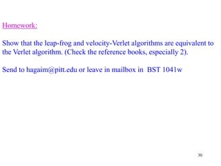
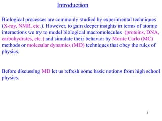
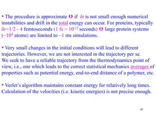
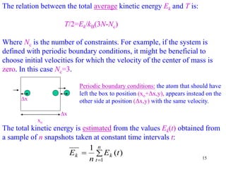
The velocities (required for the kinetic energy and temperature) are:
)
(
2
/
)]
(
)
(
[
)
( t
t
t
t
t
t 





 r
r
v
i.e., correct up to (δt)2 . They can also be estimated at half step, t+(1/2)δt,
t
t
t
t
t
t 





 /
)]
(
)
(
[
)
2
1
( r
r
v
The process is iterative. Starts with initial coordinates and velocities;
then t+δt  t and t  t- δt etc. Irrespective of initial conditions the
particles get mixed according the laws of statistical mechanics.
Most of computer time is spent on calculation of the forces, f = a/m.
The Verlet algorithm satisfies time reversal r(t + δt) = r(t - δt).

10. 10
• The procedure is approximate  if δt is not small enough numerical
instabilities and drift in the total energy can occur. For proteins, typically
δt=1/2 - 4 femtoseconds (1 fs = 10-15 seconds)  large protein systems
(~104 atoms) are limited to ~1 ms simulations.
• Very small changes in the initial conditions will lead to different
trajectories. However, we are not interested in the trajectory per se.
We seek to have a reliable trajectory from the thermodynamics point of
view, i.e., one which leads to the correct statistical mechanics averages of
properties such as potential energy, end-to-end distance of a polymer, etc.
• Verlet’s algorithm maintains constant energy for relatively long times.
Calculation of the velocities (i.e. kinetic energies) is not precise enough.

11. 11
Many other algorithms have been developed. Some are equivalent to
Verlet’s method - leap-frog (Hockney, 1970) and velocity Verlet (Swope,
Andersen, Berens& Wilson, 1982), where v is more accurate
)]
(
)
(
[
2
)
(
)
(
)
(
)
(
)
(
2
1
)
(
)
(
)
(
)
( 2
t
t
t
t
t
t
t
t
t
t
t
t
t
t















a
a
v
v
a
v
r
r
Here, first r(t+ δt) is calculated from v(t) and a(t). v(t+ δt ) is calculated
in two stages, first at mid-step, i.e., v(t+ δt/2)
)
(
2
)
(
)
(
)
2
1
( t
t
t
t
t a
v
v





Finally, a(t+ δt) is calculated and the corresponding force, which lead to
v(t+ δt)
)
(
2
)
(
)
2
1
(
)
( t
t
t
t
t
t
t 







 a
v
v

12. 12
MD and statistical mechanics
The argon atoms in the isolated box (i.e., of constant energy, Etot) are
described in statistical mechanics by a microcanonical ensemble; each
system configuration (xN,vN ) = (x1,..,xN,v1,…,vN) has the same
probability and total energy, Etot. One can calculate ensemble averages
of potential & kinetic energy < Ep> + <Ek>=Etot in phase space, ΩE(tot)
One can calculate in this ensemble the distribution of the velocity
component, vx of atom i (with mass m); it is the Maxwell-Boltzmann
(Gaussian) probability (T – temperature; kB - Boltzmann const.)



















T
k
mv
T
k
m
v
p x
x
B
2
2
/
1
B 2
1
exp
2
)
( T
k
v
m x
B
2
2
1
2




N
N
N
N
E
d
d
E
E
E
v
x
v
x )
,
(
1
tot
tot
p
p 





13. 13
The microcanonical ensemble provides a static probabilistic picture,
while MD defines a deterministic dynamical picture. In other words,
with MD (like in real experiments) measurements are carried out in time
and it would be beneficial if the two pictures could be reconciled, i.e., if
the MD time averages would lead to the ensemble averages.
Under the ergodic hypothesis a long MD run does not depend on the
initial conditions and it leads to the ensemble averages. For Ep,
Where the bar denotes time average and the brackets ensemble average.
In practice, an MD trajectory after equilibration visits only a very limited
part of phase space, consisting, however, of typical coordinates and
velocities. The velocities are distributed Maxwell Boltzmann, which
constitutes a criterion to check that equilibration has occurred.


 




p
t
N
p
p E
t
E
t
d
t
E
t
)
,
(
1
lim
0
r

14. 14
1 2
A starting non-typical a typical random
configuration configuration at high T

While the probability of (x1,..,xN,v1,…,vN) of picture 1 is equal to that of
picture 2, the number of randomly distributed configurations (as in 2) is
much larger than the cluster-like conf. of fig. 1; therefore, after
equilibration the system will “always” be found in a typical (random)
configuration (2) and the ensemble averages will be obtained.
Calculation of temperature
In a microcanonical system (N,V,E constant - V volume) T can be
defined after MD equilibration, using the relation, T =<mv2>/kB> for one
degree of freedom or from the total kinetic energy.

15. 15
The relation between the total average kinetic energy Ek and T is:
T/2=Ek/kB(3N-Nc)
Where Nc is the number of constraints. For example, if the system is
defined with periodic boundary conditions, it might be beneficial to
choose initial velocities for which the velocity of the center of mass is
zero. In this case Nc=3.
Periodic boundary conditions: the atom that should have
left the box to position (xo+Δx,y), appears instead on the
other side at position (Δx,y) with the same velocity.
Δx
xo
Δx
The total kinetic energy is estimated from the values Ek(t) obtained from
a sample of n snapshots taken at constant time intervals t:



n
t
k
k t
E
n
E
1
)
(
1

16. 16
Efficiency
• MD is a robust method, which is used extensively in all kinds of
systems, fluids, polymers, biological macromolecules etc.
• In an MD simulation two successive snapshots at times t and t+Δt are
correlated if Δt is not large enough. If the correlations are strong the
system will not span the required regions in phase space and the averages
calculated will be incorrect, i.e., the ergodic assumption unsatisfied.
• Indeed, in many cases, such as in glasses, systems under a phase
transition, and proteins, the correlations are strong even for very large Δt
and sophisticated techniques are required to handle such systems.
• Processes in nature (e.g., protein folding) and in experiments might
occur on relatively large time scales (seconds and above) that are beyond
the reach of MD with the present computers (nano - microseconds).

17. 17
Movie
216 argon atoms run by velocity Verlet algorithm at constant energy
(NVE).
Temperature 200 K (Tcritical 150 K) – dense gas.
Time step δt= 5 femtoseconds
Each frame is taken after 20 time steps (0.1 ps)
Total run time for 2500 frames is 250 ps.
To demonstrate the independence of the equilibrium behavior on the
initial conditions (ergodic theorem) the simulation starts from a non-
typical configuration where the atoms are arranged at the corner with a
density of liquid argon (i.e., 8 times higher than the system density after
equilibration).

18. 18
Potential Energy as a Function of Time
-250
-200
-150
-100
-50
0
0 20 40 60 80 100
time (ps)
Potential
Energy
(kcal/mol)
Potential energy calculated from the movie frames

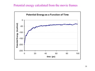
19. 19
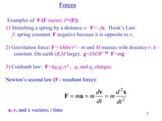
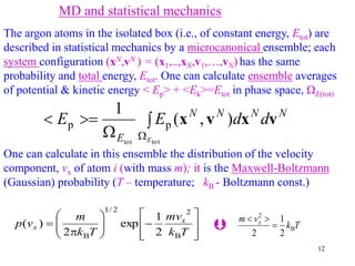
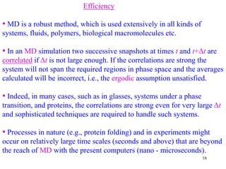
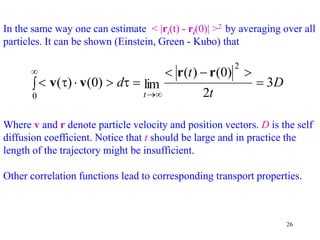
Fluctuations in Total Energy for an NVE Simulation of
216 TIP3P Water Molecules (1fs time step)
[the run was initiated at E = -1730.32 kcal/mol]
-1730.5
-1730.45
-1730.4
-1730.35
-1730.3
-1730.25
-1730.2
0 10000 20000 30000 40000 50000
time (ps)
Total
Energy
(kcal/mol)

20. 20
Snapshots of Kinetic Energy for an NVE Simulation of
216 TIP3P Water Molecules (1fs time step)
<Kinetic Energy> = 384.1 kcal/mol (of systems)
= 1.778 kcal/mol (of molecules)
= (6/2)RT therefore T = 298K
300
350
400
450
500
0 10000 20000 30000 40000 50000
time (ps)
Kinetic
Energy
(kcal/mol)

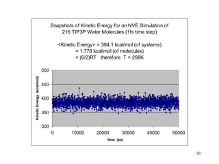
21. 21
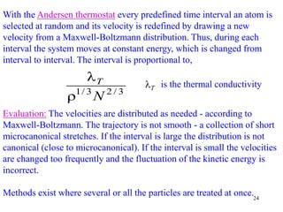
Snapshots of Potential Energy for an NVE Simulation of
216 TIP3P Water Molecules (1fs time step)
<Potential Energy> = -2114.4 kcal/mol (of systems)
= -9.789 kcal/mol (of molecules) [exp. = -9.92 kcal/mol]
-2180
-2160
-2140
-2120
-2100
-2080
-2060
0 10000 20000 30000 40000 50000
time (ps)
Potential
Energy
(kcal/mol)

22. 22
MD simulations in the canonical ensemble
As we have seen, in the microcanonical ensmble (N,V,E), an MD run is
completely mechanistic. However, in the canonical ensemble, where the
temperature, T replaces the energy, E (i.e.,the variables are N,V,T) one
has to provide a “thermostat”, i.e., a procedure to keep T constant. The
most common thermostats are those of Berendsen and Andersen.
In the canonical ensemble the system is in contact with a large (infinite)
heat bath with constant Tbath, which exchanges energy with the system.
At equilibrium the average temperature of the system is also Tbath, but
this temperature slightly fluctuates around its average value (Tbath), the
larger the system the smaller the fluctuations. According to the
Berendsen thermostat at each time step the velocities are rescaled by the
factor
δt - time step
tT - parameter
2
/
1
sysem
bath
1
1





















T
T
t
t
T

23. 23
For one degree of freedom assuming δt = tT one obtains
For δt < tT the change in velocities is more moderate and tT = 0.4 ps has
been found to be appropriate.
Evaluation: easy to implement, works well, but doest not obey the
canonical distribution (the velocities are not distributed according to
Maxwell-Boltzmann). This procedure can lead to local hot and cold
regions in the system while Tsystem is ok, i.e. Tsystem ~Tbath.
bath
B
sysem
bath
system
B
2
system
B
2
2
1
1 T
k
T
T
T
k
T
k
mv 























24. 24
With the Andersen thermostat every predefined time interval an atom is
selected at random and its velocity is redefined by drawing a new
velocity from a Maxwell-Boltzmann distribution. Thus, during each
interval the system moves at constant energy, which is changed from
interval to interval. The interval is proportional to,
3
/
2
3
/
1
N
T

 is the thermal conductivity
T

Evaluation: The velocities are distributed as needed - according to
Maxwell-Boltzmann. The trajectory is not smooth - a collection of short
microcanonical stretches. If the interval is large the distribution is not
canonical (close to microcanonical). If the interval is small the velocities
are changed too frequently and the fluctuation of the kinetic energy is
incorrect.
Methods exist where several or all the particles are treated at once.

25. 25
Dynamics
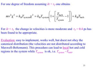
MD not only provides statistical mechanics averages, but also allows
calculating dynamical properties. One can calculate from an MD
trajectory time correlation functions that lead to dynamic parameters
such as diffusion coefficients. For example, the autocorrelation function
of the velocity


 )
(
)
0
( t
i
i v
v
can be estimated from an MD trajectory, where the velocities are
measured n times in time intervals t
In practice, the measurements start at time (m+1)t and go back m time
intervals. Contribution from all particles are considered and averaged.
 











N
i
i
i
n
m
k
i
i t
m
k
kt
N
m
n
mt
1
1
]
)
[(
]
[
)
1
(
1
)
(
)
0
( v
v
v
v

26. 26
In the same way one can estimate < |ri(t) - ri(0)| >2 by averaging over all
particles. It can be shown (Einstein, Green - Kubo) that
D
t
t
d
t
3
2
)
0
(
)
(
lim
)
0
(
)
(
2
0








 



 r
r
v
v
Where v and r denote particle velocity and position vectors. D is the self
diffusion coefficient. Notice that t should be large and in practice the
length of the trajectory might be insufficient.
Other correlation functions lead to corresponding transport properties.

27. 27
Biological macromolecules - proteins
The typical potential energy function (force field) is:
EFF = bonds Kr(r - req)2 + angles K( - eq)2
+ dihedrals Vn /2 [1 + cos(n - )]
+ i<j [Aij /Rij
12 – Bij /Rij
6 + qiqj /Rij]
where Kr , K , req, eq, , n, Vn, Aij, Bij, and qi are parameters
optimized by applying this function to a large amount of experimental
data and results obtained from quantum mechanical ab initio
calculations.
Rij is the distance between atoms i and j and  is a dielectric constant.
A protein in vacuum – no solvent effects - the screening of the Coulomb
potentials by water can partially be obtained by increasing .
Rij

r

28. 28
Typically the protein is immersed in a ‘box’ of water molecules where
the system consists of n ~10,000 atoms (or more). Most of computer
time is spent on calculating the forces related to water-water protein-
protein and water-protein interactions.
Notice that the “spring constants” Kr and K are strong (leading to fast
motions) and would require small time step, δt ,  relatively short
trajectories. Therefore, in most studies part or all of the bond lengths are
constrained by procedures such as SHAKE and RATTLE.
For proteins MD is significantly more efficient than Monte Carlo (MC)
techniques, because with MD the atoms move according the calculated
forces while with MC the atomic positions are changed at random which
leads to high energy structures that are rejected in the process.

29. 29
In an MD simulation of a protein at room temperature the system can
get trapped for a long simulation time in the potential energy well of the
starting structure and the move to more stable parts of conformational
space is extremely slow, unreachable within a feasible simulation time.
This problem can somewhat be resolved by methods such as parallel
tempering, which is a hybrid of MD and MC.
Ep
conformations
initial well
most stable well
barriers

30. 30
Homework:
Show that the leap-frog and velocity-Verlet algorithms are equivalent to
the Verlet algorithm. (Check the reference books, especially 2).
Send to hagaim@pitt.edu or leave in mailbox in BST 1041w