Download as PDF, PPTX
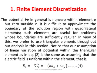
![Step 6:
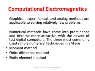
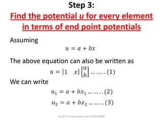
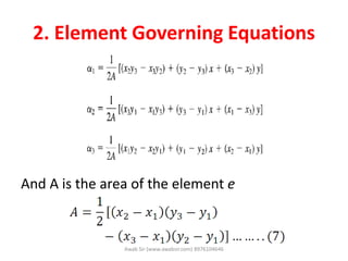
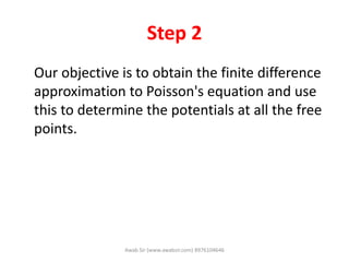
Obtain the general solution
The matrix [K] is a function of geometry and
the material properties. The curly brackets
denote column matrix. Equation 9 does not
lead to a unique solution. For a unique
solution we have to apply boundary
conditions.
Awab Sir (www.awabsir.com) 8976104646](https://image.slidesharecdn.com/module04computationalelectromagnetics-140417132421-phpapp01/85/Computational-electromagnetics-18-320.jpg)
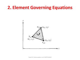
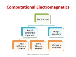
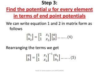
![3. Assembling of all Elements
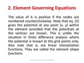
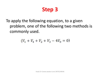
Having considered a typical element, the next step is to
assemble all such elements in the solution region. The
energy associated with the assemblage of all elements
in the mesh is
Where n is the number of nodes,
N is the number of elements, and
[C] is called the overall or global coefficient matrix, which
is the assemblage of individual element coefficient
matrices.
Awab Sir (www.awabsir.com) 8976104646](https://image.slidesharecdn.com/module04computationalelectromagnetics-140417132421-phpapp01/85/Computational-electromagnetics-38-320.jpg)
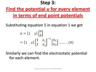
![3. Assembling of all Elements
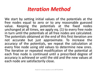
The properties of matrix [C] are
1. It is symmetric (Cij = Cji) just as the element
coefficient matrix.
2. Since Cij = 0 if no coupling exists between
nodes i and j, it is evident that for a large
number of elements [C] becomes sparse and
banded.
3. It is singular.
Awab Sir (www.awabsir.com) 8976104646](https://image.slidesharecdn.com/module04computationalelectromagnetics-140417132421-phpapp01/85/Computational-electromagnetics-39-320.jpg)
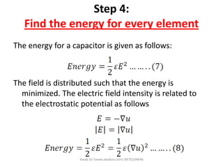
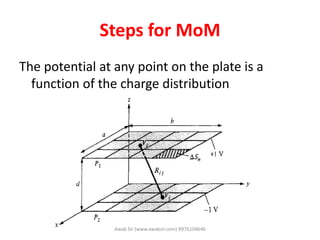
![Band Matrix Method
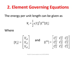
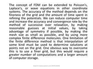
Equation (1) applied to all free nodes results in a set
of simultaneous equations of the form
Where: [A] is a sparse matrix (i.e., one having many
zero terms),
[V] consists of the unknown potentials at the free
nodes, and
[B] is another column matrix formed by the known
potentials at the fixed nodes.
Awab Sir (www.awabsir.com) 8976104646](https://image.slidesharecdn.com/module04computationalelectromagnetics-140417132421-phpapp01/85/Computational-electromagnetics-54-320.jpg)
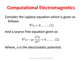
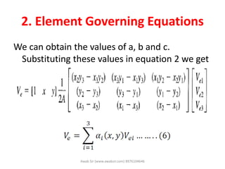
![Band Matrix Method
Matrix [A] is also banded in that its nonzero
terms appear clustered near the main
diagonal because only nearest neighboring
nodes affect the potential at each node. The
sparse, band matrix is easily inverted to
determine [V]. Thus we obtain the potentials
at the free nodes from matrix [V] as
Awab Sir (www.awabsir.com) 8976104646](https://image.slidesharecdn.com/module04computationalelectromagnetics-140417132421-phpapp01/85/Computational-electromagnetics-55-320.jpg)
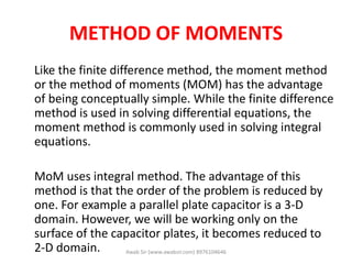
![Step 3
Assuming there is uniform charge distribution on each
subsection we get
This equation can be rearranged to obtain
Where, [B]: column matrix defining the potentials
[A]: square matrix
In MoM, the potential at any point is the function of
potential distribution at all points, this was not done in
FDM and FEM. Awab Sir (www.awabsir.com) 8976104646](https://image.slidesharecdn.com/module04computationalelectromagnetics-140417132421-phpapp01/85/Computational-electromagnetics-62-320.jpg)
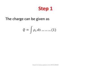
![Finite Difference
Method (FDM)
Finite Element Method
(FEM)
Method of Moments
(MoM)
Basic
principle
Based on differentiation
i.e. the differential
equation is converted to a
difference equation.
1. Energy based (energy
minimization)
2. Weighted residual
(reducing the error)
Based on integral
method
Advantage 1. Simplest method
2. Taylor series based
1. Computationally easier
than MoM
2. Can be applied to
unisotropic media.
3. [K] matrix is sparse
1. More accurate
(errors effectively
tend to cancel each
other)
2. Ideally suited for
open boundary
conditions
3. Popular for
antennas
Disadvantage 1. Need to have uniform
rectangular sections
(not possible for real
life structures)
2. Outdated
1. Difficult as compared to
FDM
1. Mathematically
complex
Awab Sir (www.awabsir.com) 8976104646](https://image.slidesharecdn.com/module04computationalelectromagnetics-140417132421-phpapp01/85/Computational-electromagnetics-63-320.jpg)

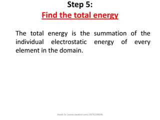
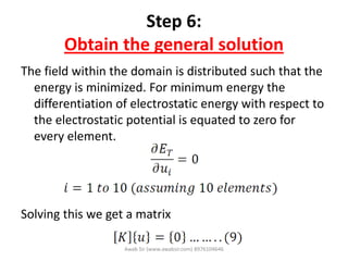
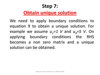
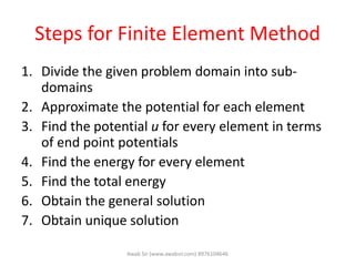
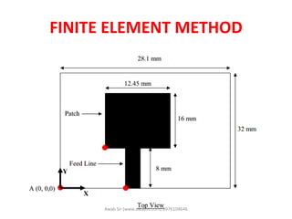
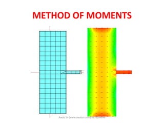
The document discusses computational electromagnetics and the finite element method. It provides 7 steps for the finite element method: 1) divide the problem domain into sub-domains, 2) approximate the potential for each element, 3) find the potential for each element in terms of end points, 4) find the energy for each element, 5) find the total energy, 6) obtain the general solution, and 7) obtain a unique solution by applying boundary conditions. The finite element method is useful for problems with complex geometries and boundary conditions that cannot be solved analytically.