Metodo degli Elementidi Contorno
Prof. Roberto Citarella
Dipartimento di Ingegneria Industriale – Università di Salerno
Gruppo di Costruzione di Macchine
2.
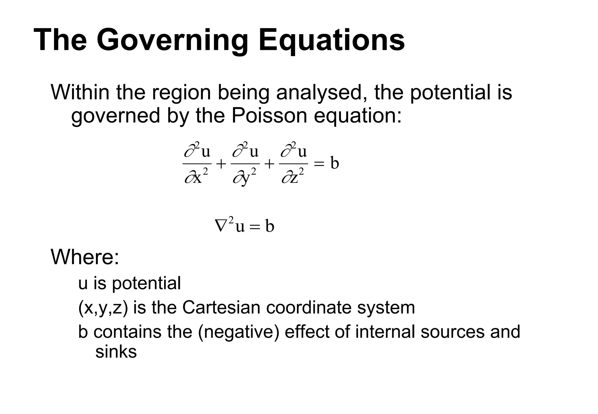
The Governing Equations
Withinthe region being analysed, the potential is
governed by the Poisson equation:
Where:
u is potential
(x,y,z) is the Cartesian coordinate system
b contains the (negative) effect of internal sources and
sinks
2
2
2
2
2
2
u
x
u
y
u
z
b
2
u b
3.
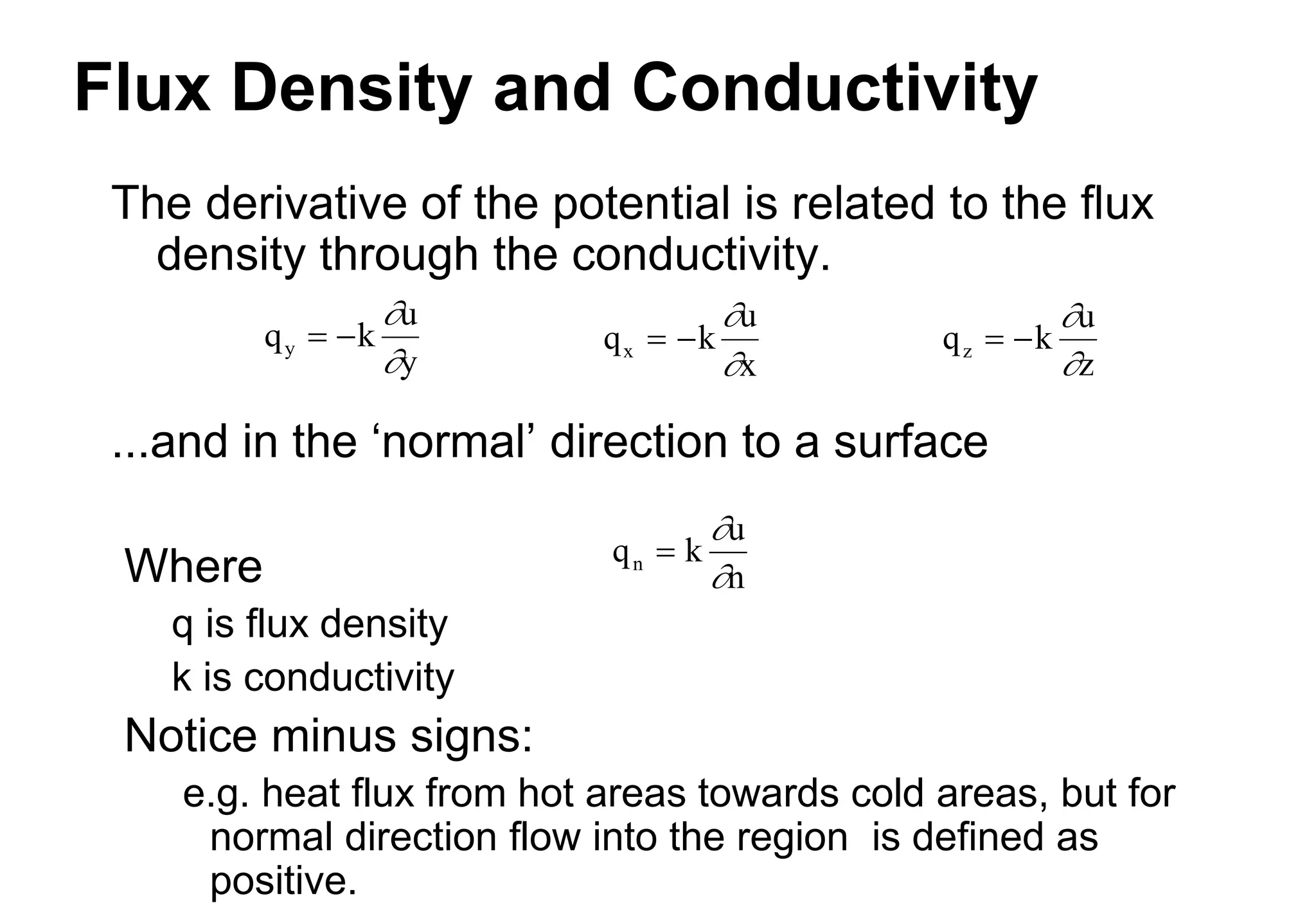
Flux Density andConductivity
The derivative of the potential is related to the flux
density through the conductivity.
...and in the ‘normal’ direction to a surface
Where
q is flux density
k is conductivity
Notice minus signs:
e.g. heat flux from hot areas towards cold areas, but for
normal direction flow into the region is defined as
positive.
q k
u
x
x
q k
u
y
y
q k
u
z
z
q k
u
n
n
4.
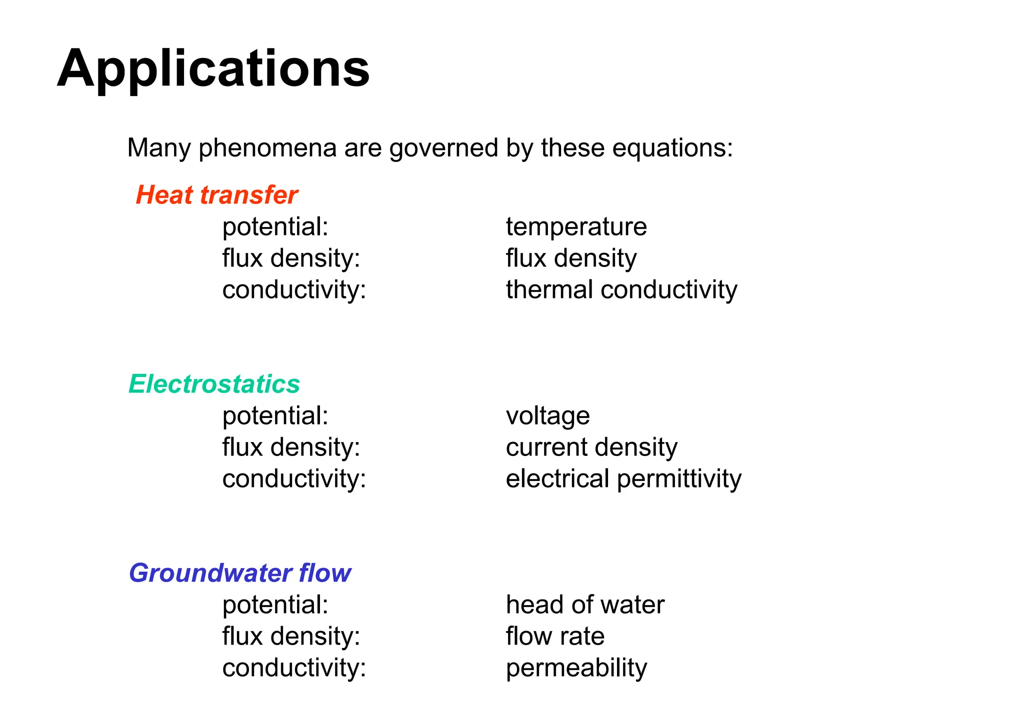
Applications
Heat transfer
potential: temperature
fluxdensity: flux density
conductivity: thermal conductivity
Electrostatics
potential: voltage
flux density: current density
conductivity: electrical permittivity
Groundwater flow
potential: head of water
flux density: flow rate
conductivity: permeability
Many phenomena are governed by these equations:
5.
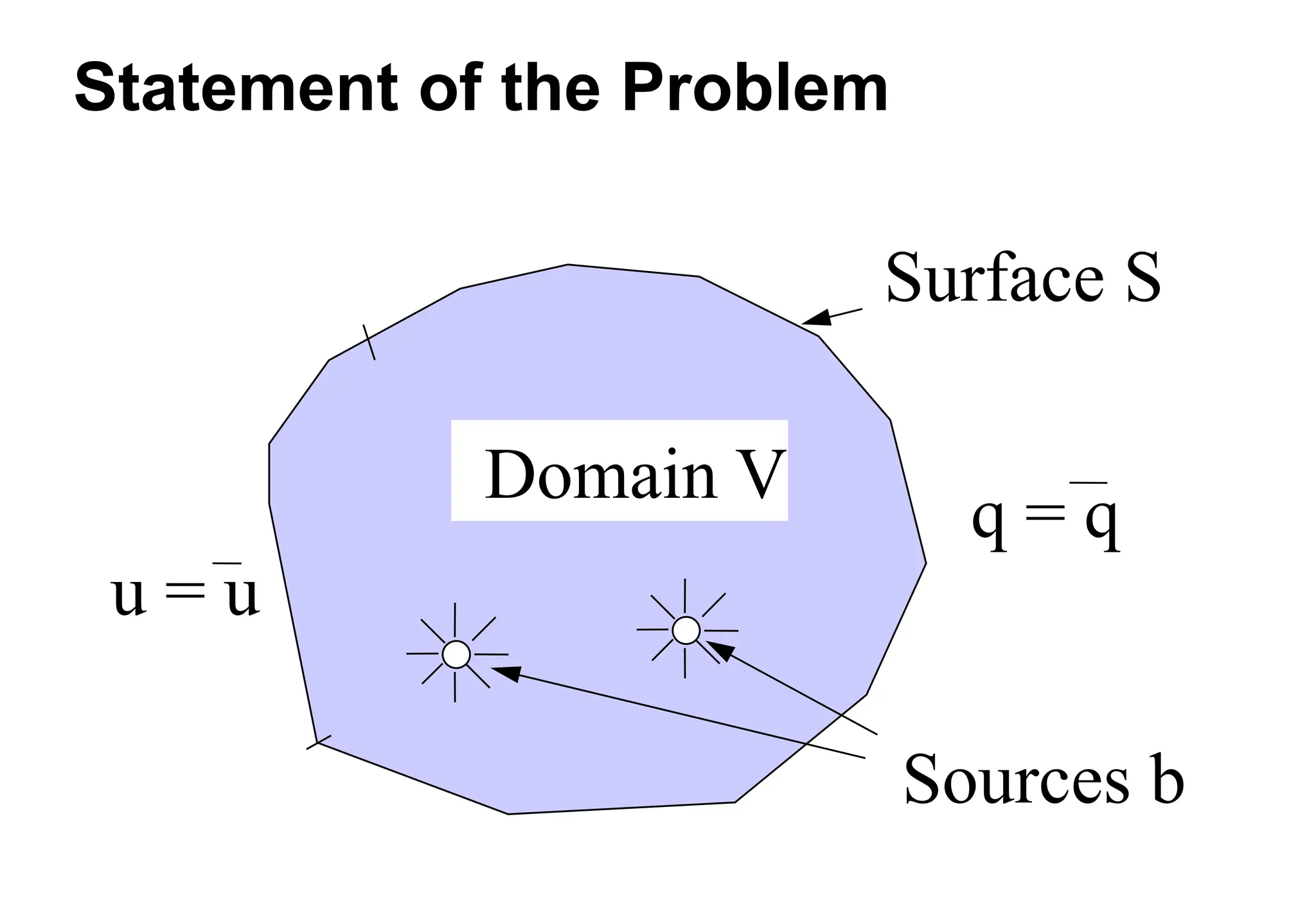
Statement of theProblem
u = u
q = q
Domain V
Surface S
Sources b
6.
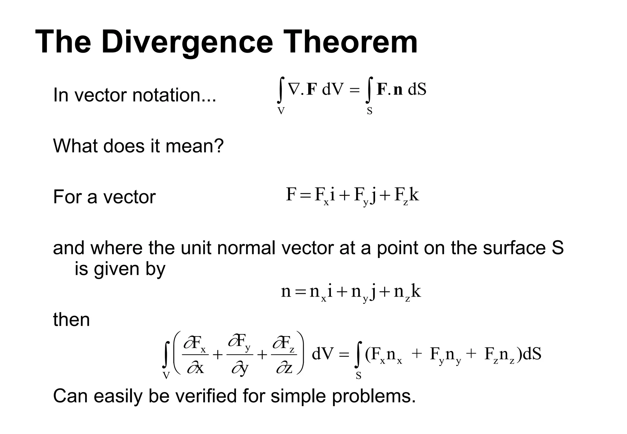
The Divergence Theorem
Invector notation...
What does it mean?
For a vector
and where the unit normal vector at a point on the surface S
is given by
then
Can easily be verified for simple problems.
. dV . dS
S
V
F F n
F
x
F
y
F
z
dV (F n + F n + F n )dS
x y z
x x y y z z
S
V
k
n
j
n
i
n
n z
y
x
k
F
j
F
i
F
F z
y
x
7.
Application of theDivergence Theorem
Considering arbitrary, differentiable functions u and u* over V, apply the divergence
theorem to the product
This gives us the expression
Similarly applying the divergence theorem to the product
gives the equation
u u * u u * dV u u*.n dS
2
V S
u* u u* u dV u* u.n dS
2
V S
*
u u
u
*
u
Subtracting one of the integral expressions from the other cancels some terms and
leaves us with...
u* u - u u* dV u* u - u u* .n dS
2
V S
2
8.
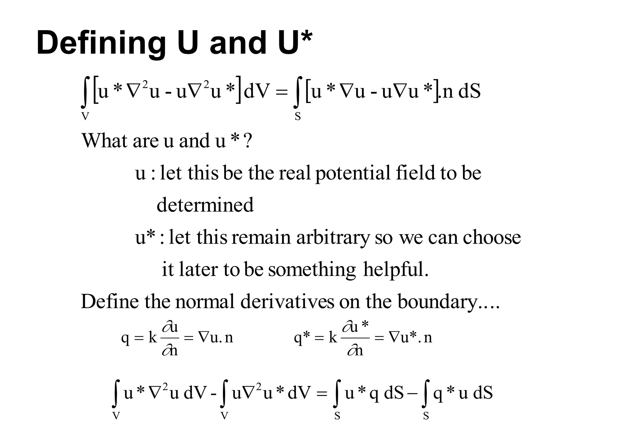
Defining U andU*
..
boundary..
on the
s
derivative
normal
the
Define
helpful.
something
be
later to
it
choose
can
we
so
arbitrary
remain
let this
:
u*
determined
be
to
field
potential
real
the
be
let this
:
u
?
*
u
and
u
are
What
dS
.n
*
u
u
-
u
*
u
dV
*
u
u
-
u
*
u
S
V
2
2
q k
u
n
u.n
q* k
u *
n
u*.n
u* u dV - u u*dV u*q dS q *u dS
2
V
2
V S S
9.
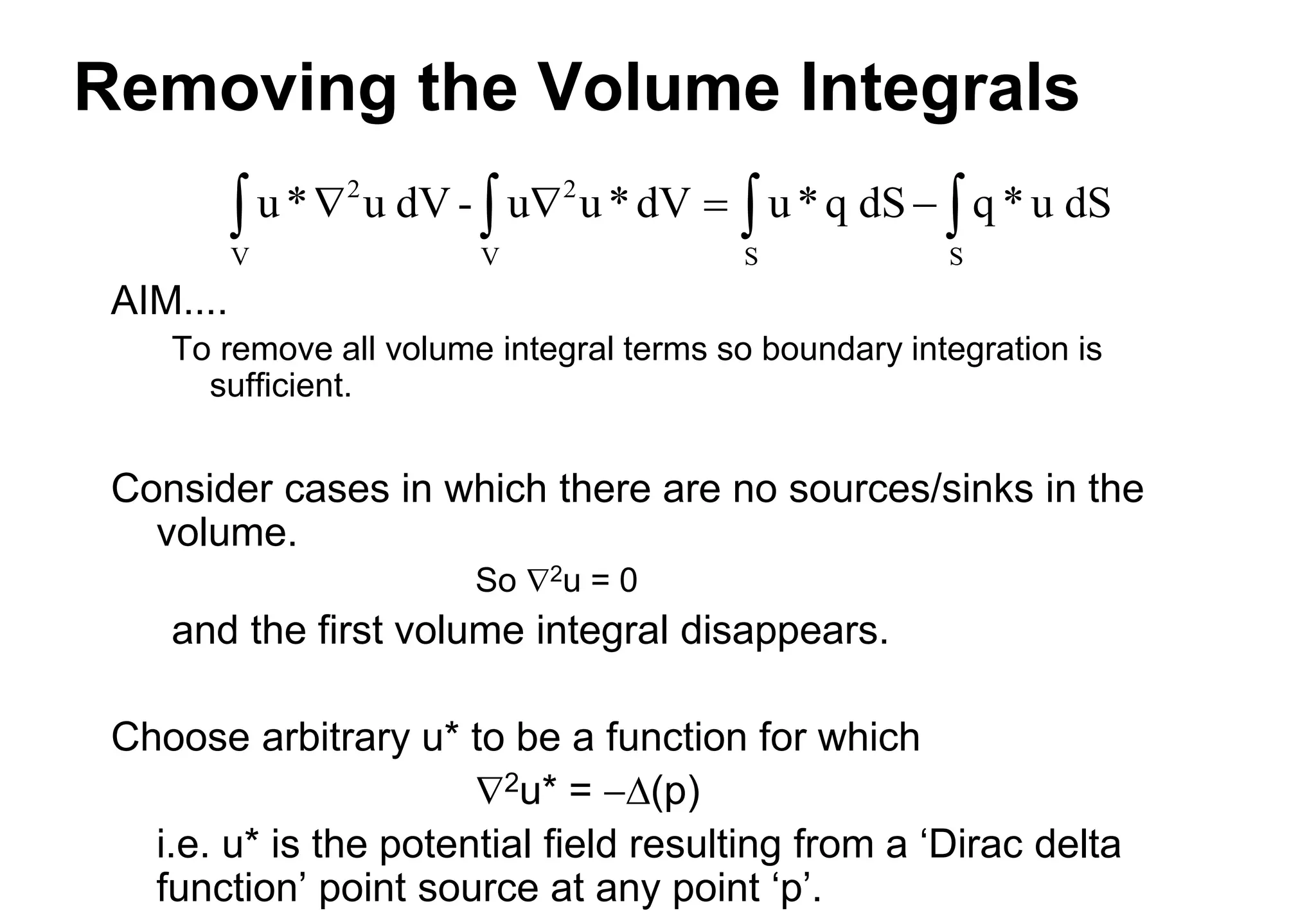
Removing the VolumeIntegrals
AIM....
To remove all volume integral terms so boundary integration is
sufficient.
Consider cases in which there are no sources/sinks in the
volume.
So 2u = 0
and the first volume integral disappears.
Choose arbitrary u* to be a function for which
2u* = D(p)
i.e. u* is the potential field resulting from a ‘Dirac delta
function’ point source at any point ‘p’.
u* u dV - u u*dV u*q dS q *u dS
2
V
2
V S S
10.
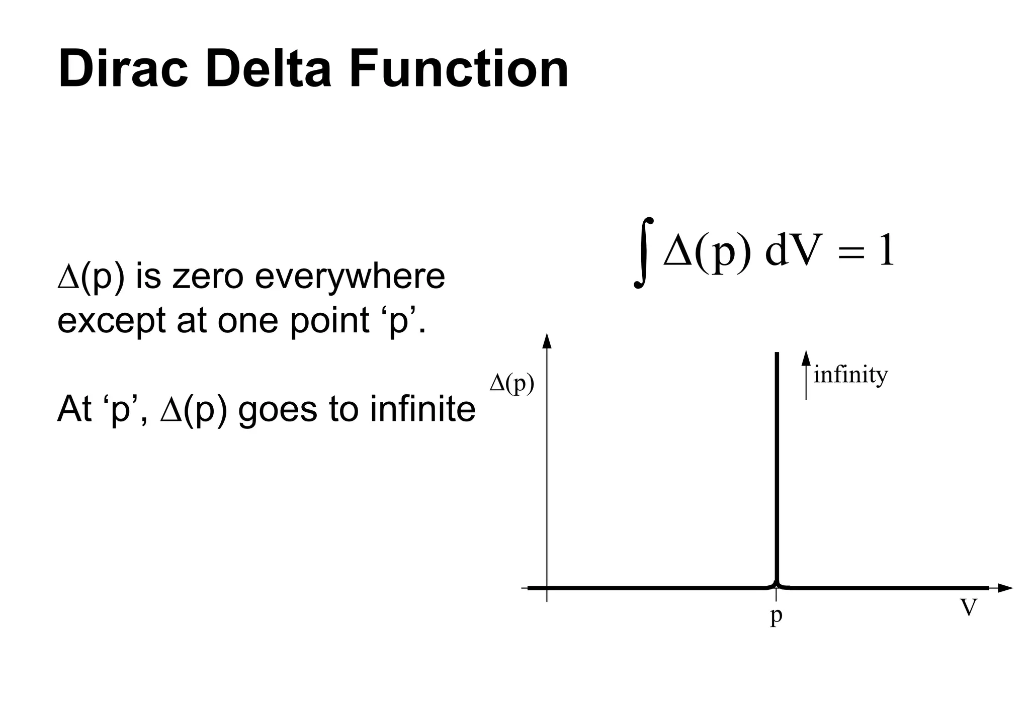
Dirac Delta Function
D(p)is zero everywhere
except at one point ‘p’.
At ‘p’, D(p) goes to infinite
D(p) dV
1
D(p) infinity
V
p
11.
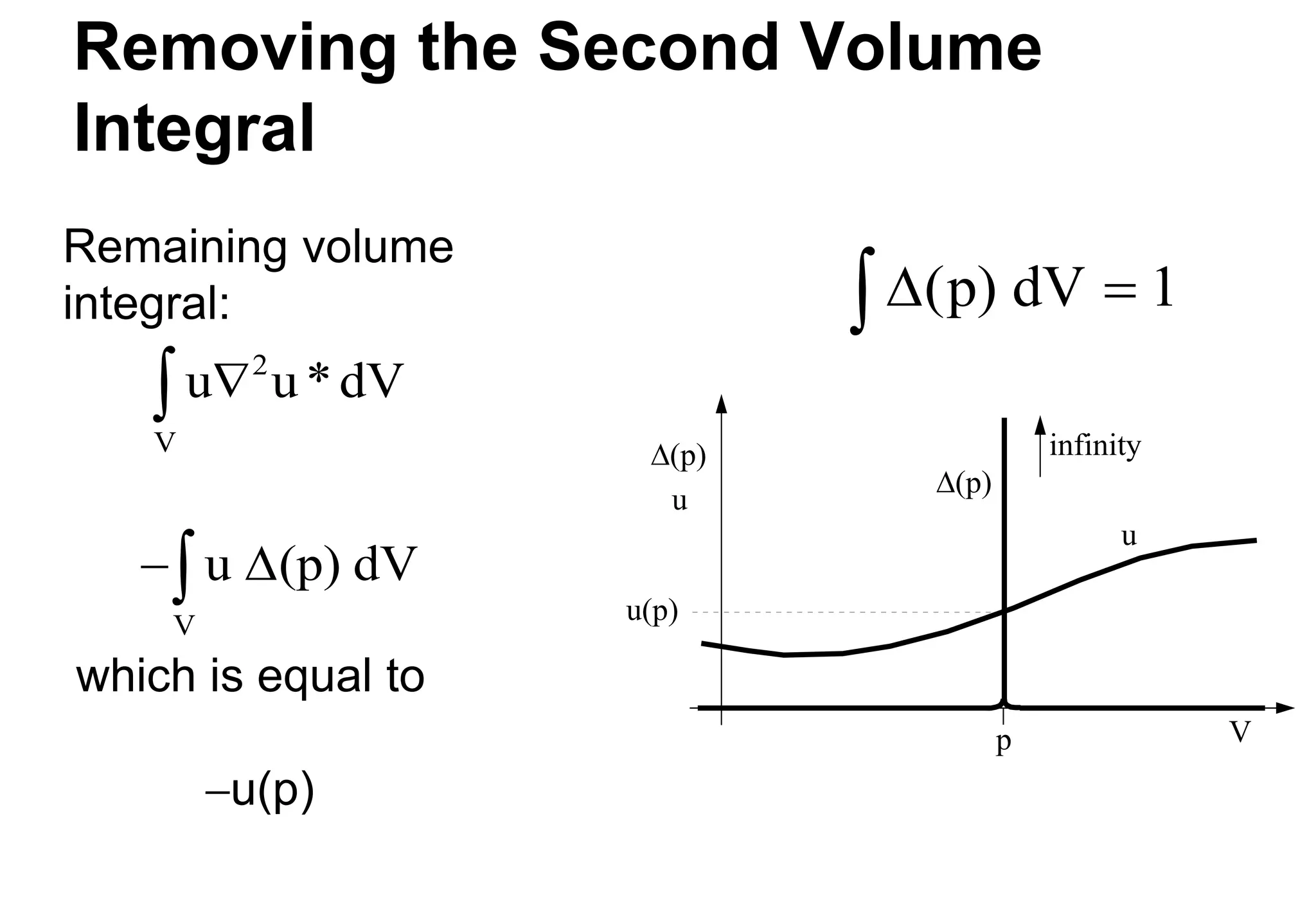
Removing the SecondVolume
Integral
Remaining volume
integral:
which is equal to
u(p)
D(p) dV
1
D(p) infinity
V
D(p)
u
u
u(p)
p
u u*dV
2
V
u (p) dV
V
D
12.
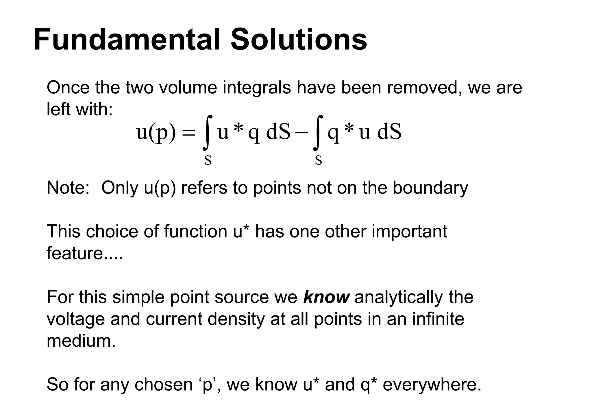
Fundamental Solutions
Once thetwo volume integrals have been removed, we are
left with:
Note: Only u(p) refers to points not on the boundary
This choice of function u* has one other important
feature....
For this simple point source we know analytically the
voltage and current density at all points in an infinite
medium.
So for any chosen ‘p’, we know u* and q* everywhere.
u(p) u*q dS q *u dS
S S
13.
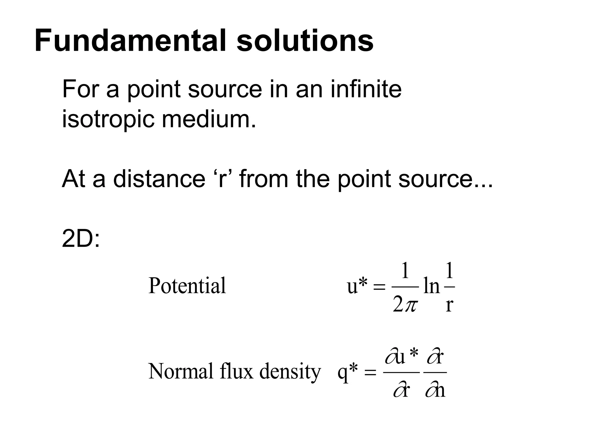
Fundamental solutions
For apoint source in an infinite
isotropic medium.
At a distance ‘r’ from the point source...
2D:
Potential u
r
* ln
1
2
1
Normal flux density q*
u*
r
r
n
14.
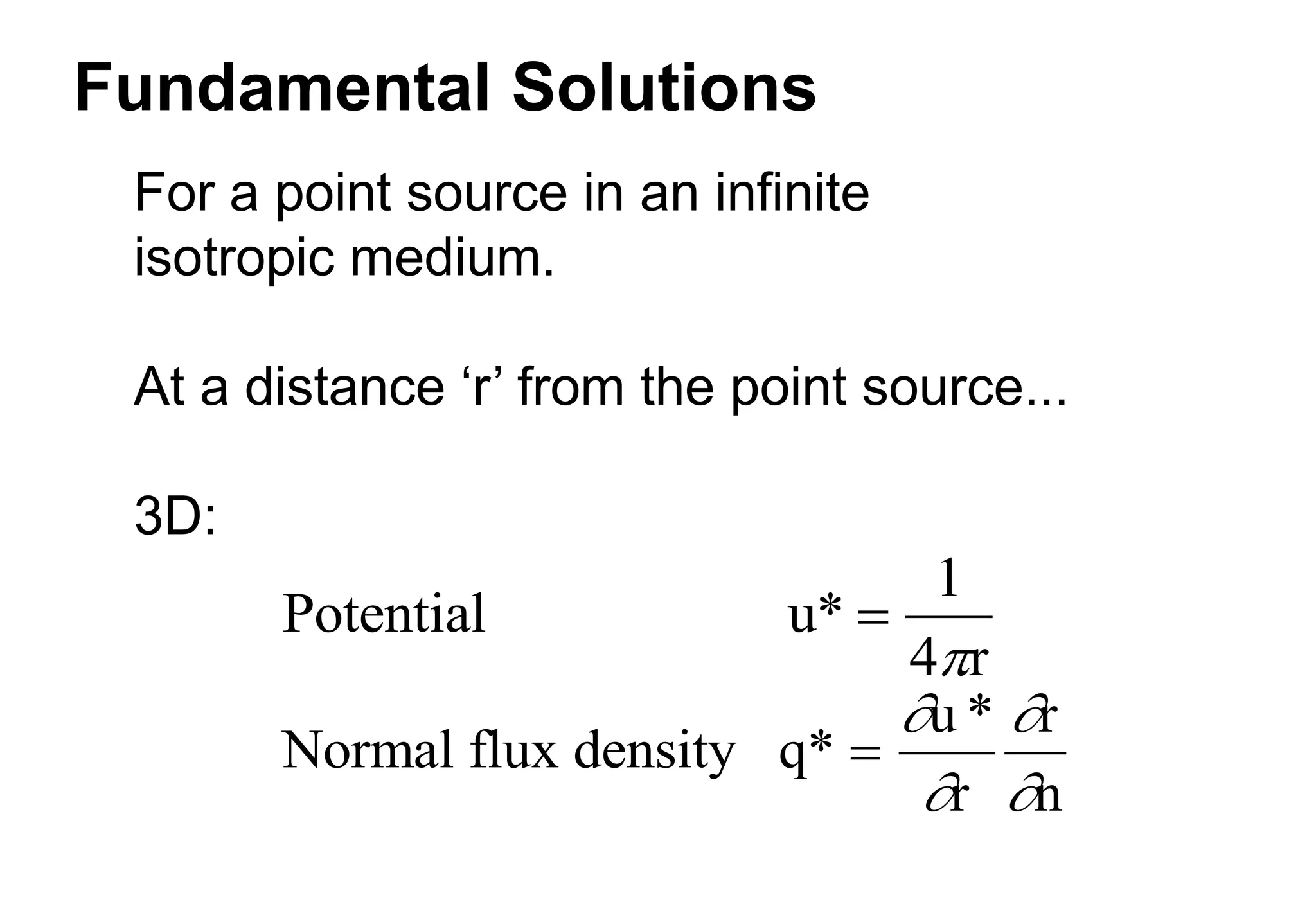
Fundamental Solutions
For apoint source in an infinite
isotropic medium.
At a distance ‘r’ from the point source...
3D:
Potential u
r
*
1
4
Normal flux density q*
u *
r
r
n
15.
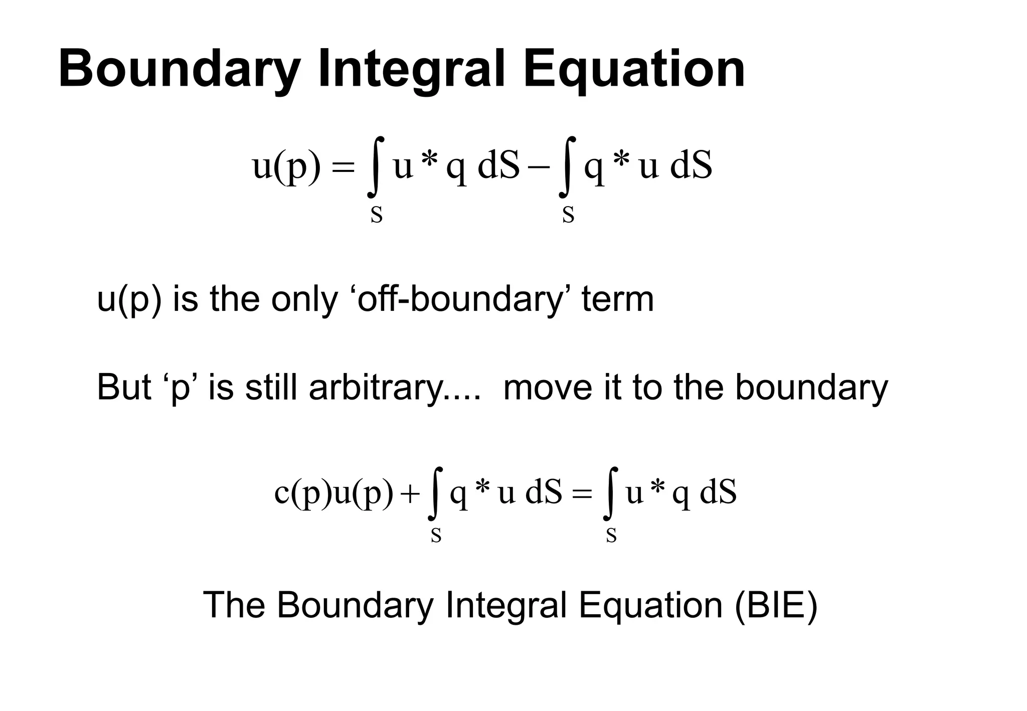
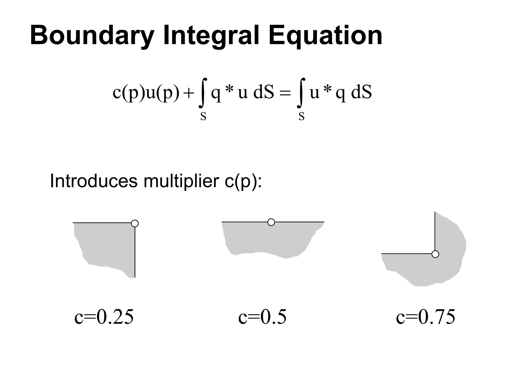
Boundary Integral Equation
u(p)is the only ‘off-boundary’ term
But ‘p’ is still arbitrary.... move it to the boundary
u(p) u*q dS q *u dS
S S
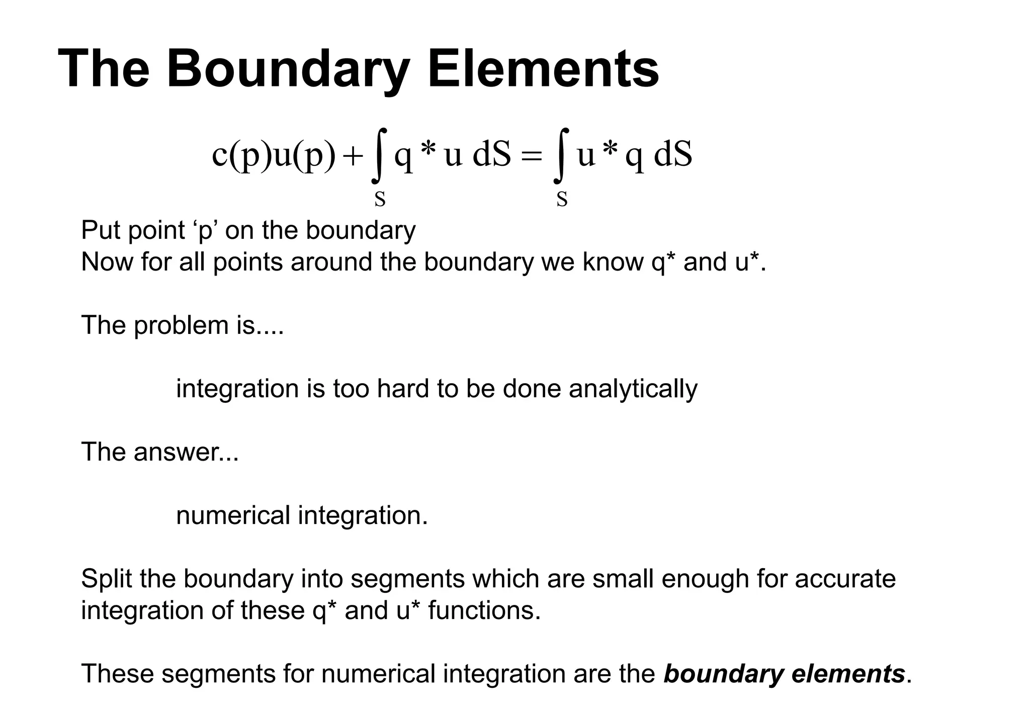
The Boundary Integral Equation (BIE)
c(p)u(p) q * u dS u*q dS
S S
The Boundary Elements
Putpoint ‘p’ on the boundary
Now for all points around the boundary we know q* and u*.
The problem is....
integration is too hard to be done analytically
The answer...
numerical integration.
Split the boundary into segments which are small enough for accurate
integration of these q* and u* functions.
These segments for numerical integration are the boundary elements.
c(p)u(p) q * u dS u*q dS
S S
18.
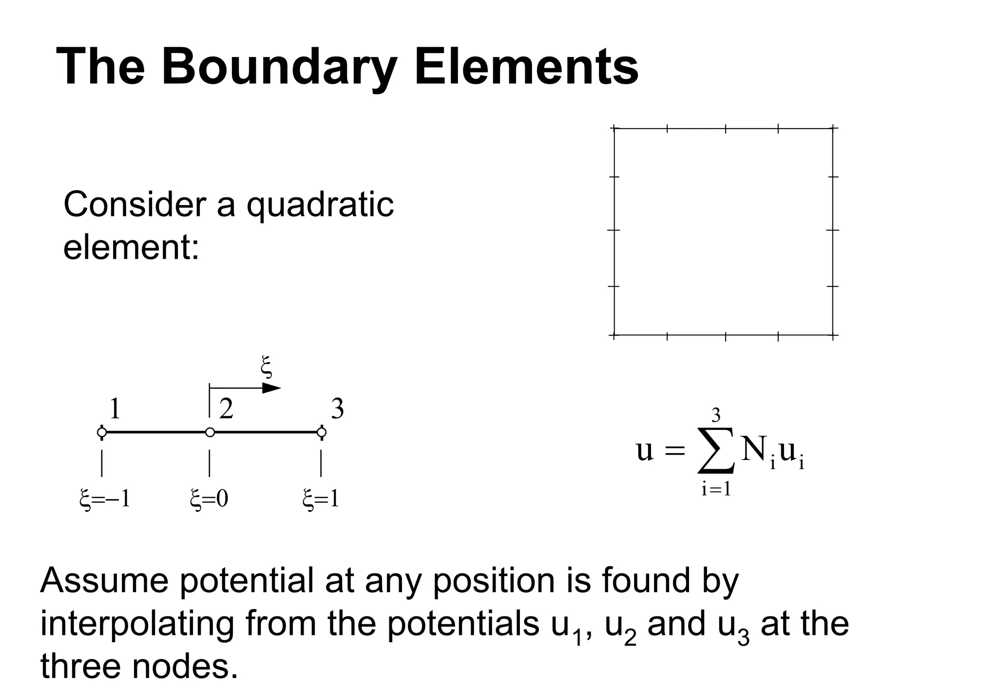
The Boundary Elements
Assumepotential at any position is found by
interpolating from the potentials u1, u2 and u3 at the
three nodes.
1 2 3
u N u
i
i 1
3
i
Consider a quadratic
element:
19.
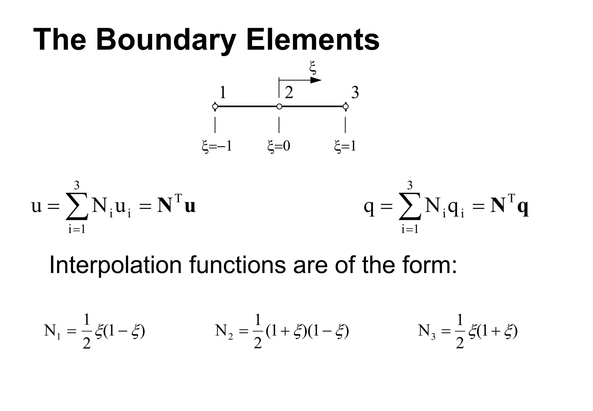
The Boundary Elements
Interpolationfunctions are of the form:
1 2 3
u N u
i
i 1
3
i
T
N u q N q
i
i 1
3
i
T
N q
N1
1
2
1
( ) N2
1
2
1 1
( )( )
N3
1
2
1
( )
20.
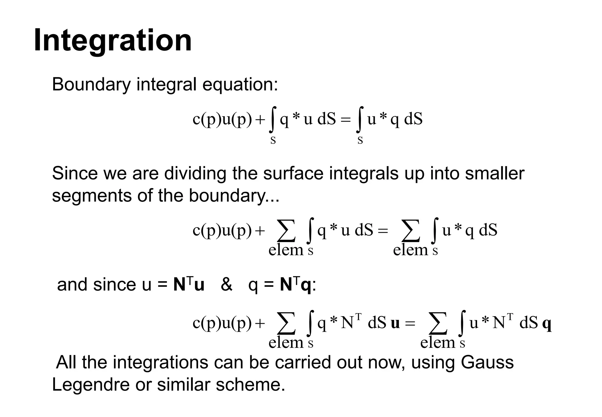
Integration
Boundary integral equation:
Sincewe are dividing the surface integrals up into smaller
segments of the boundary...
and since u = NTu & q = NTq:
All the integrations can be carried out now, using Gauss
Legendre or similar scheme.
c(p)u(p) q * u dS u*q dS
S S
c(p)u(p) q *u dS
elem
u*q dS
elem
S S
c(p)u(p) q *N dS
elem
u*N dS
elem
T
S
T
S
u q
21.
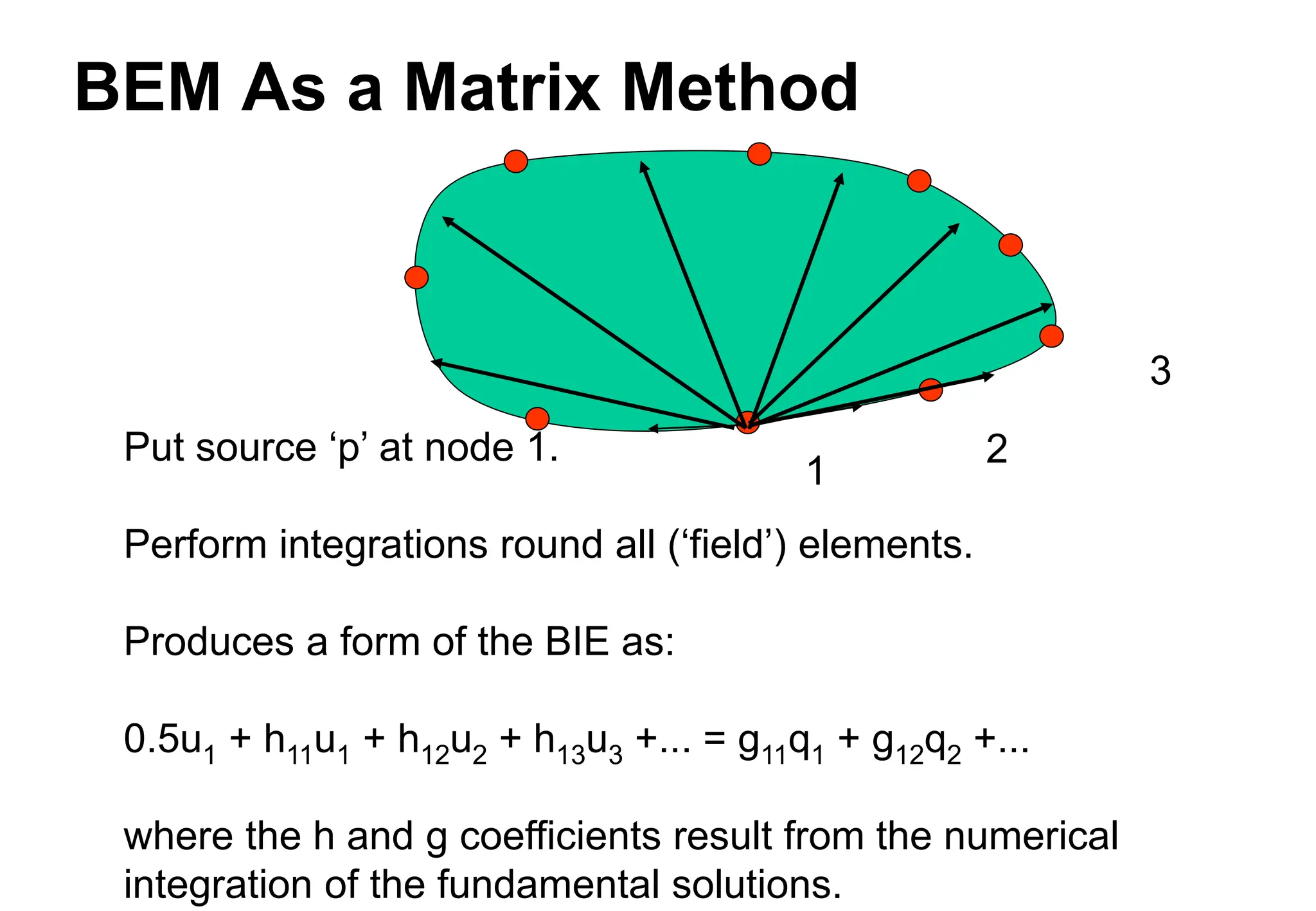
BEM As aMatrix Method
Put source ‘p’ at node 1.
Perform integrations round all (‘field’) elements.
Produces a form of the BIE as:
0.5u1 + h11u1 + h12u2 + h13u3 +... = g11q1 + g12q2 +...
where the h and g coefficients result from the numerical
integration of the fundamental solutions.
1
2
3
22.
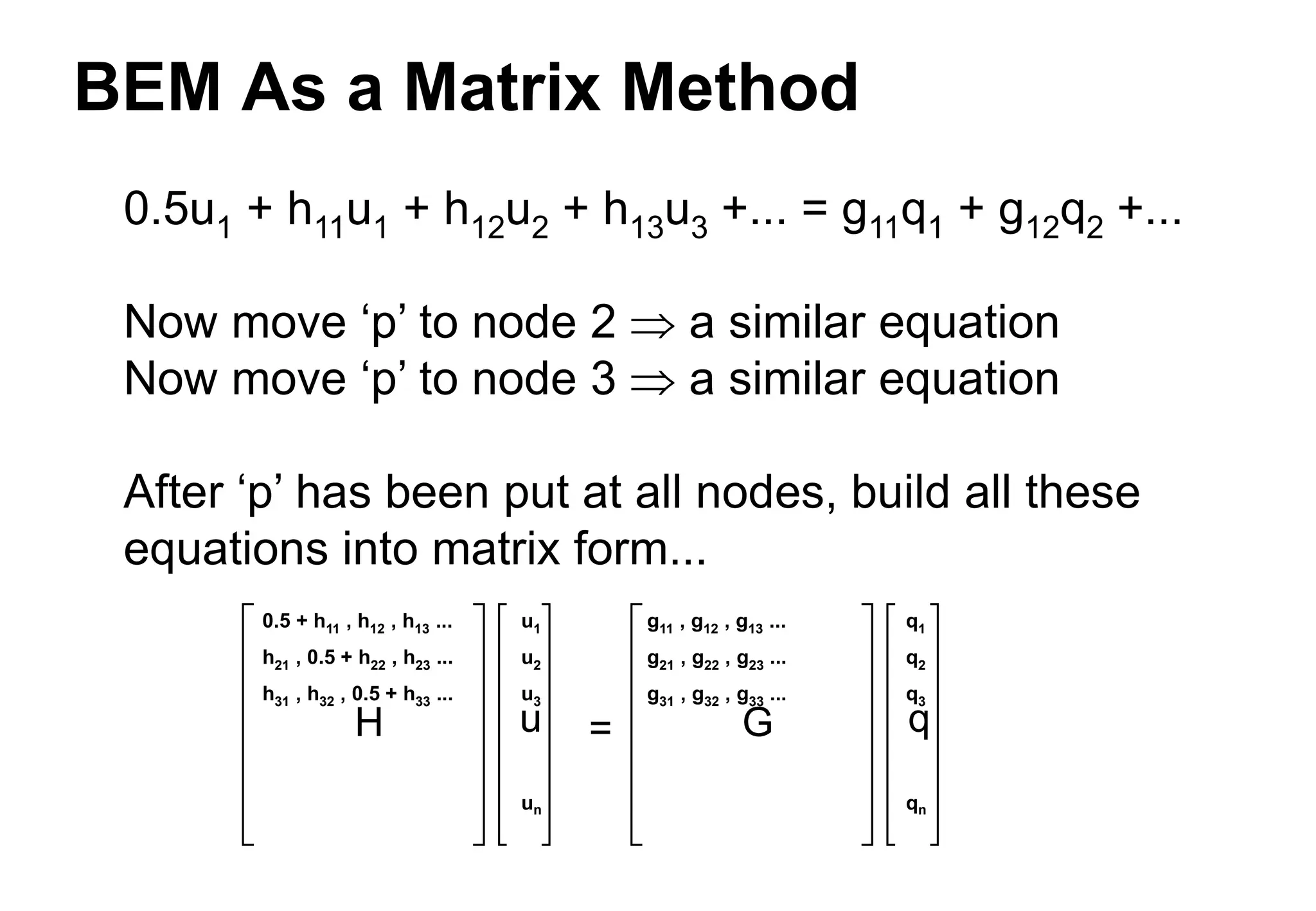
BEM As aMatrix Method
0.5u1 + h11u1 + h12u2 + h13u3 +... = g11q1 + g12q2 +...
Now move ‘p’ to node 2 a similar equation
Now move ‘p’ to node 3 a similar equation
After ‘p’ has been put at all nodes, build all these
equations into matrix form...
H u G q
=
0.5 + h11 , h12 , h13 ...
h21 , 0.5 + h22 , h23 ...
h31 , h32 , 0.5 + h33 ...
g11 , g12 , g13 ...
g21 , g22 , g23 ...
g31 , g32 , g33 ...
u1
u2
u3
un
q1
q2
q3
qn
23.
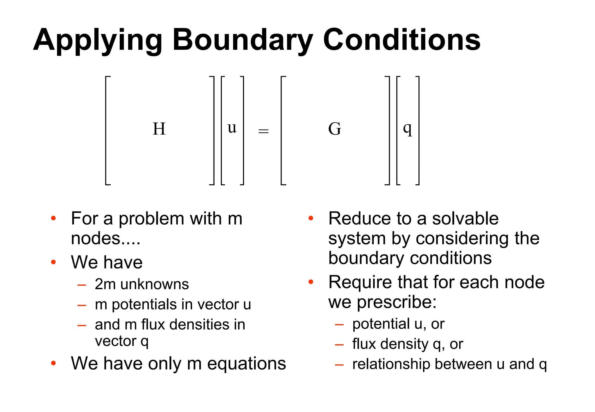
Applying Boundary Conditions
•For a problem with m
nodes....
• We have
– 2m unknowns
– m potentials in vector u
– and m flux densities in
vector q
• We have only m equations
• Reduce to a solvable
system by considering the
boundary conditions
• Require that for each node
we prescribe:
– potential u, or
– flux density q, or
– relationship between u and q
H u G q
=
24.
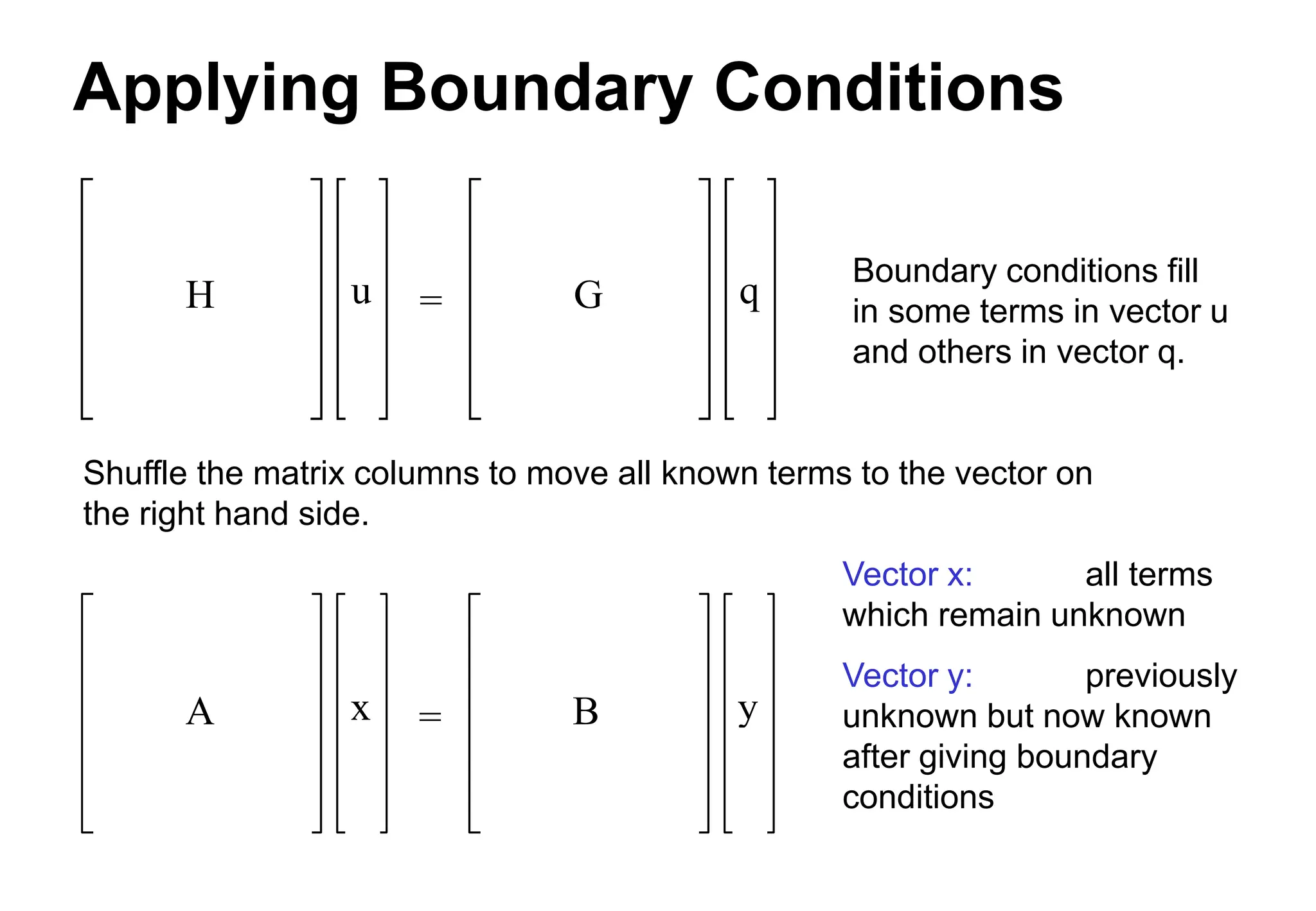
Applying Boundary Conditions
Shufflethe matrix columns to move all known terms to the vector on
the right hand side.
H u G q
=
A x B y
=
Vector x: all terms
which remain unknown
Vector y: previously
unknown but now known
after giving boundary
conditions
Boundary conditions fill
in some terms in vector u
and others in vector q.
25.
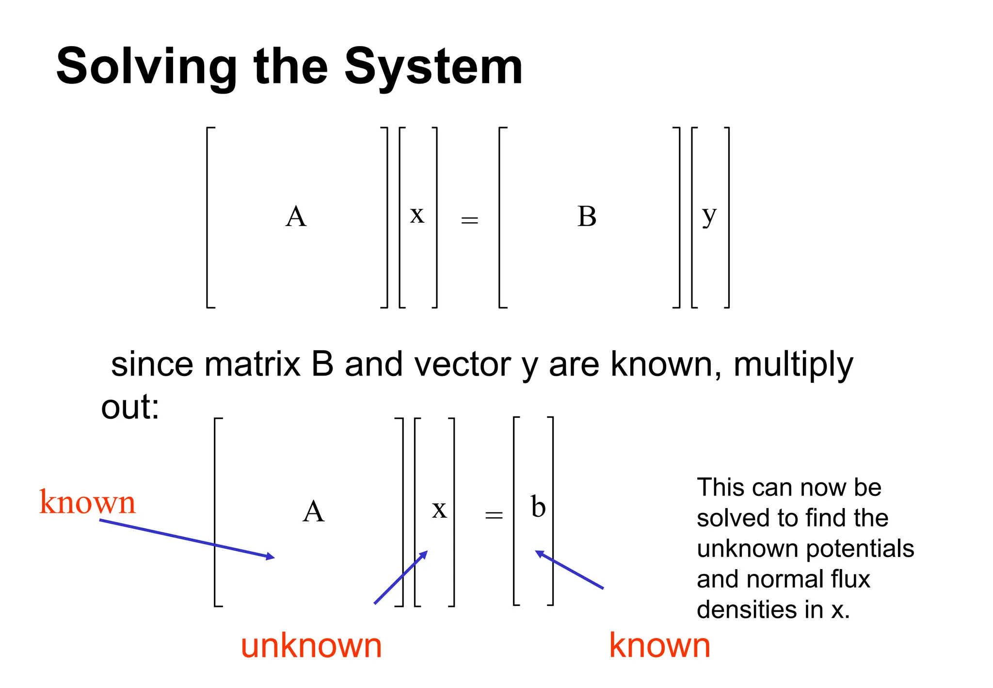
Solving the System
known
sincematrix B and vector y are known, multiply
out:
A x B y
=
A x b
=
This can now be
solved to find the
unknown potentials
and normal flux
densities in x.
known
unknown
26.
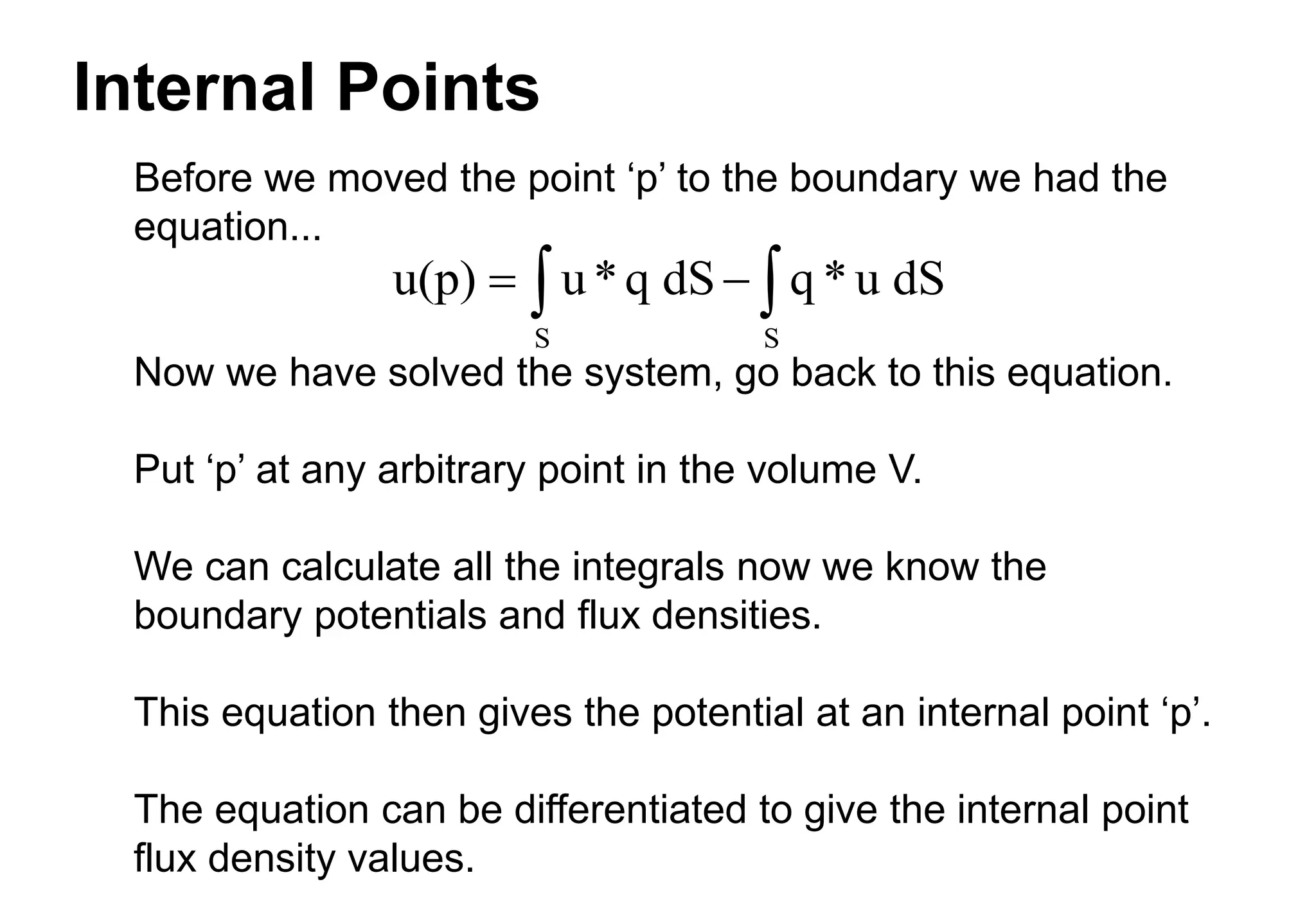
Internal Points
Before wemoved the point ‘p’ to the boundary we had the
equation...
Now we have solved the system, go back to this equation.
Put ‘p’ at any arbitrary point in the volume V.
We can calculate all the integrals now we know the
boundary potentials and flux densities.
This equation then gives the potential at an internal point ‘p’.
The equation can be differentiated to give the internal point
flux density values.
u(p) u*q dS q *u dS
S S
27.
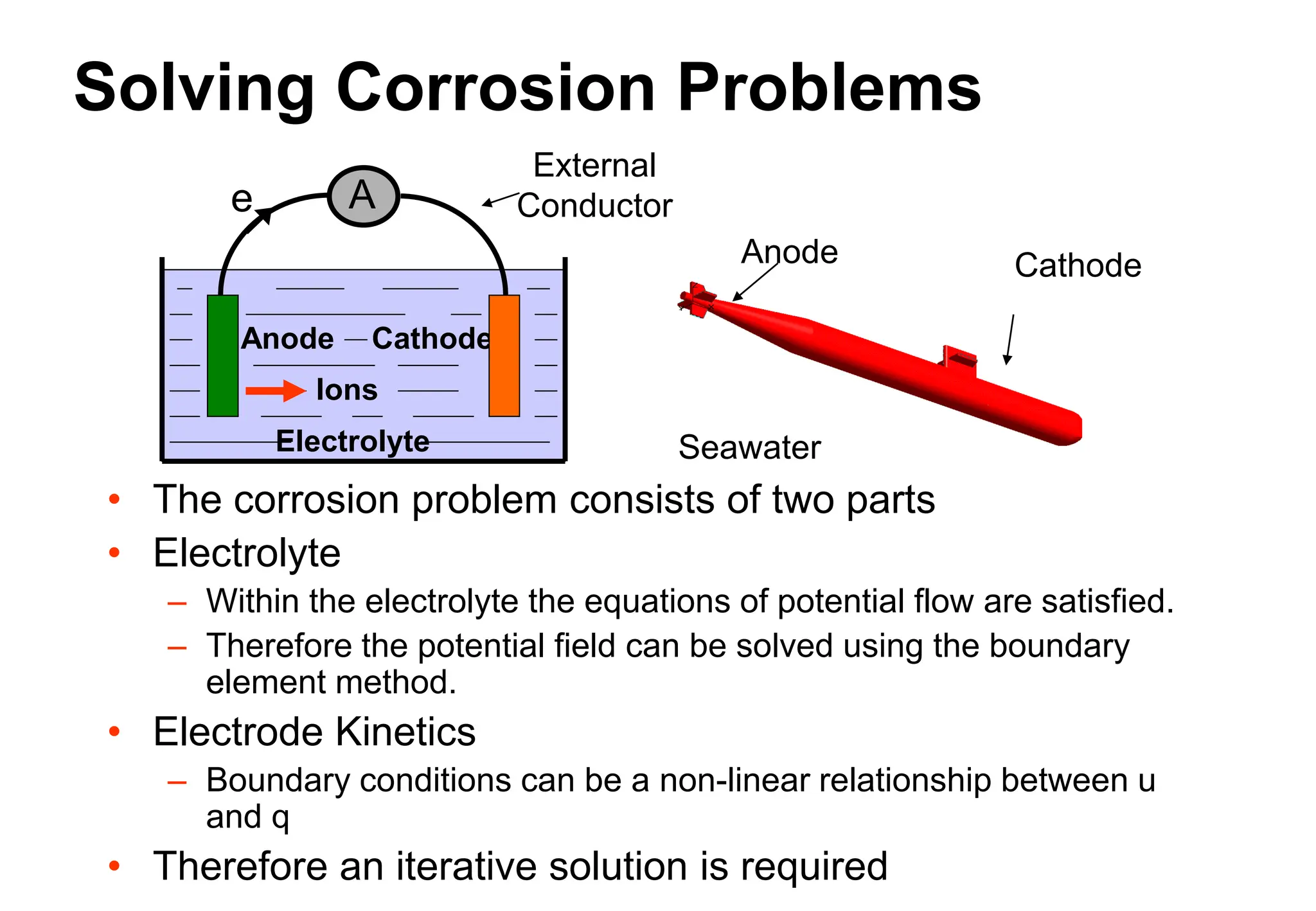
Solving Corrosion Problems
•The corrosion problem consists of two parts
• Electrolyte
– Within the electrolyte the equations of potential flow are satisfied.
– Therefore the potential field can be solved using the boundary
element method.
• Electrode Kinetics
– Boundary conditions can be a non-linear relationship between u
and q
• Therefore an iterative solution is required
Seawater
Anode Cathode
External
Conductor
Anode Cathode
Ions
A
Electrolyte
e
28.
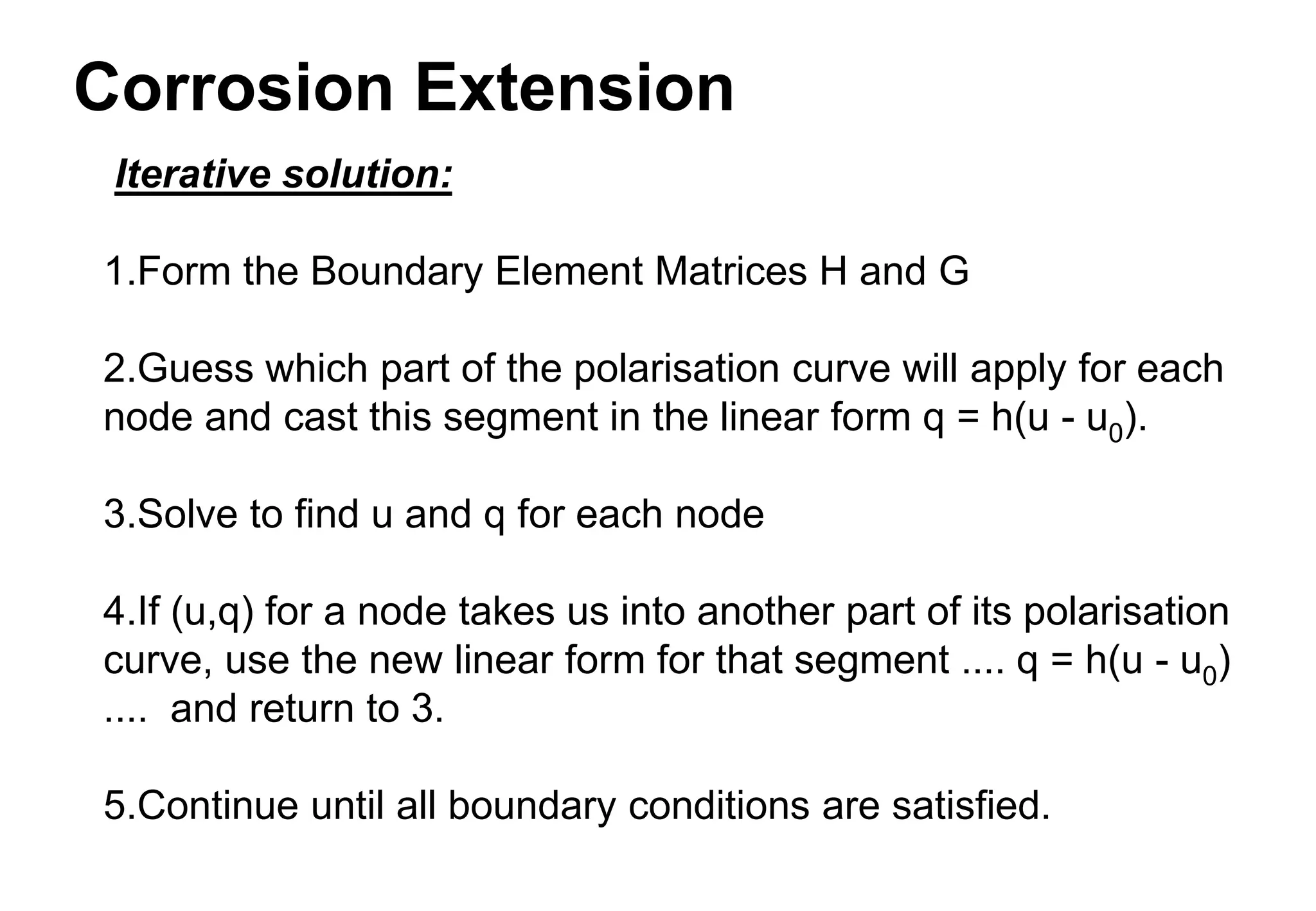
Corrosion Extension
Iterative solution:
1.Formthe Boundary Element Matrices H and G
2.Guess which part of the polarisation curve will apply for each
node and cast this segment in the linear form q = h(u - u0).
3.Solve to find u and q for each node
4.If (u,q) for a node takes us into another part of its polarisation
curve, use the new linear form for that segment .... q = h(u - u0)
.... and return to 3.
5.Continue until all boundary conditions are satisfied.