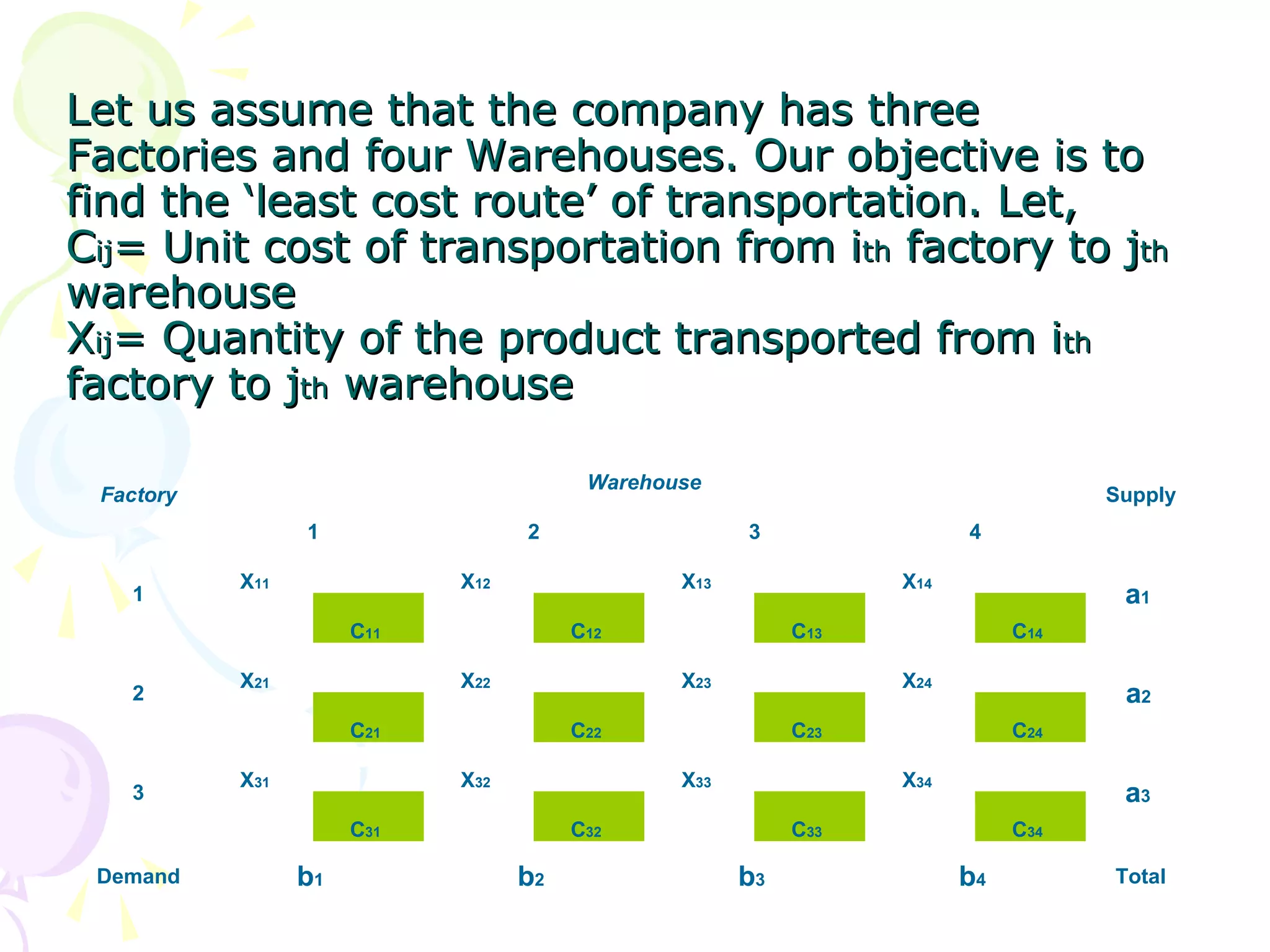
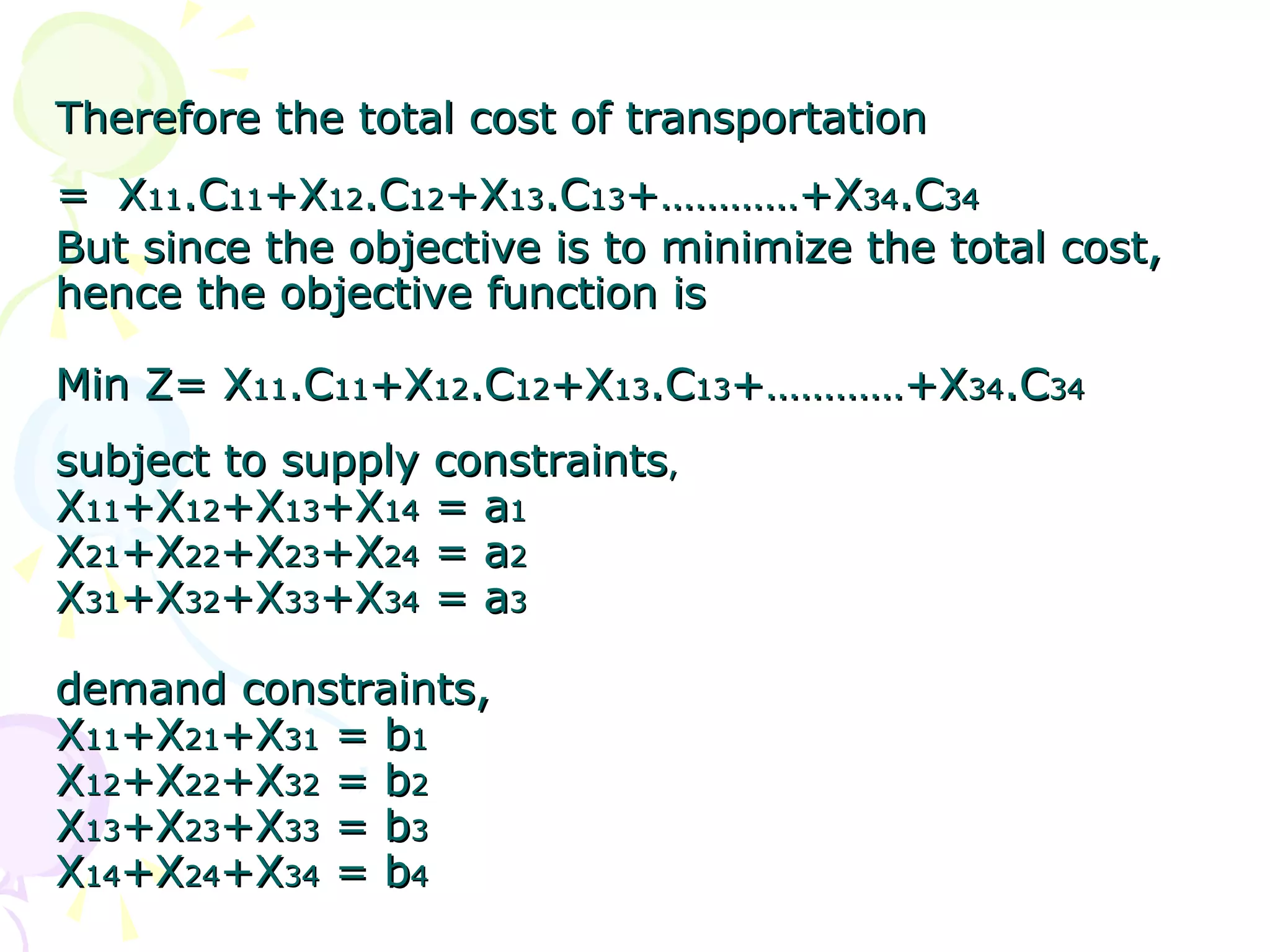
This document discusses transportation models and methods for finding an initial basic feasible solution and testing for optimality in transportation problems. It describes three methods - northwest corner, least cost, and Vogel's approximation - for obtaining an initial solution. It then explains how to test if the initial solution is optimal using the MODI or u-v method by calculating opportunity costs for unoccupied cells and finding a closed path if any cells have negative opportunity costs to obtain an improved solution. The process repeats until all opportunity costs are non-negative, indicating an optimal solution.

1. TRANSPORTATIONTRANSPORTATION
PROBLEMPROBLEM
Shubhagata RoyShubhagata Roy
School of Management SciencesSchool of Management Sciences
VaranasiVaranasi

2. Concept of Transportation ModelsConcept of Transportation Models
Transportation is a O.R. technique intended toTransportation is a O.R. technique intended to
establish the ‘least cost route’ of transportation ofestablish the ‘least cost route’ of transportation of
goods from the company’s factories to itsgoods from the company’s factories to its
warehouses located at different places.warehouses located at different places.
It is a special type of linear programming problemIt is a special type of linear programming problem
(LPP) that involves transportation or physical(LPP) that involves transportation or physical
distribution of goods and services from supply pointsdistribution of goods and services from supply points
(factories) to the demand points (warehouses). The(factories) to the demand points (warehouses). The
problem involves determination of optimum routes toproblem involves determination of optimum routes to
minimize shipping costs from supply source tominimize shipping costs from supply source to
destinations.destinations.

3. Let us assume that the company has threeLet us assume that the company has three
Factories and four Warehouses. Our objective is toFactories and four Warehouses. Our objective is to
find the ‘least cost route’ of transportation. Let,find the ‘least cost route’ of transportation. Let,
CCijij= Unit cost of transportation from i= Unit cost of transportation from ithth factory to jfactory to jthth
warehousewarehouse
XXijij= Quantity of the product transported from i= Quantity of the product transported from ithth
factory to jfactory to jthth warehousewarehouse
Factory
Warehouse
Supply
1 2 3 4
1
X11 X12 X13 X14
a1
C11 C12 C13 C14
2
X21 X22 X23 X24
a2
C21 C22 C23 C24
3
X31 X32 X33 X34
a3
C31 C32 C33 C34
Demand b1 b2 b3 b4 Total

4. Therefore the total cost of transportationTherefore the total cost of transportation
== XX1111.C.C1111+X+X1212.C.C1212+X+X1313.C.C1313+…………+X+…………+X3434.C.C3434
But since the objective is to minimize the total cost,But since the objective is to minimize the total cost,
hence the objective function ishence the objective function is
Min Z= XMin Z= X1111.C.C1111+X+X1212.C.C1212+X+X1313.C.C1313+…………+X+…………+X3434.C.C3434
subject to supply constraintssubject to supply constraints,,
XX1111+X+X1212+X+X1313+X+X1414 = a= a11
XX2121+X+X2222+X+X2323+X+X2424 = a= a22
XX3131+X+X3232+X+X3333+X+X3434 = a= a33
demand constraints,demand constraints,
XX1111+X+X2121+X+X3131 = b= b11
XX1212+X+X2222+X+X3232 = b= b22
XX1313+X+X2323+X+X3333 = b= b33
XX1414+X+X2424+X+X3434 = b= b44

5. Initial Basic FeasibleInitial Basic Feasible
SolutionSolution
1.1.North-West Corner Method (NWCM)North-West Corner Method (NWCM)
2.2.Least Cost Method (LCM)Least Cost Method (LCM)
3.3.Vogel’s Approximation Method (VAM)Vogel’s Approximation Method (VAM)

6. North-West Corner MethodNorth-West Corner Method
Step1: Select the upper left (north-west) cell of the
transportation matrix and allocate minimum of supply and
demand, i.e., min.(a1,b1) value in that cell.
Step2:
• If a1< b1, then allocation made is equal to the supply
available at the first source (a1 in first row), then move
vertically down to the cell (2,1).
• If a1> b1, then allocation made is equal to demand of the
first destination (b1 in first column), then move horizontally
to the cell (1,2).
• If a1=b1 , then allocate the value of a1 or b1 and then move
to cell (2,2).
Step3: Continue the process until an allocation is made in
the south-east corner cell of the transportation table.

7. ExampleExample:: Solve the Transportation Table to find InitialSolve the Transportation Table to find Initial
Basic Feasible Solution using North-West Corner Method.Basic Feasible Solution using North-West Corner Method.
Total Cost =19*5+30*2+30*6+40*3+70*4+20*14Total Cost =19*5+30*2+30*6+40*3+70*4+20*14
= Rs. 1015= Rs. 1015
Supply
19 30 50 10
5 2
70 30 40 60
6 3
40 8 70 20
4 14
Demand 34
S1
S2
S3
7
9
18
D1 D2 D3 D4
5 8 7 14

8. Least Cost MethodLeast Cost Method
Step1: Select the cell having lowest unit cost in the entire
table and allocate the minimum of supply or demand values
in that cell.
In case, the smallest unit cost is not unique, then select the
cell where maximum allocation (allocation process will be
same as discussed before) can be made.
Step2: Then eliminate the row or column in which supply or
demand is exhausted. If both the supply and demand
values are same, either of the row or column can be
eliminated.
Step3: Repeat the process with next lowest unit cost and
continue until the entire available supply at various sources
and demand at various destinations is satisfied.

9. Supply
70
2
40
3
Demand 345
S2 2
S3 3
D1
Supply
70 40 60
40 70 20
7
Demand 34
S3 10
5 7 7
S2 9
D1 D3 D4
Supply
70 40
7
40 70
Demand 34
9
3S3
5 7
S2
D1 D3
Supply
19 30 50 10
70 30 40 60
40 8 70 20
8
Demand 34
S3 18
5 8 7 14
S1 7
S2 9
D1 D2 D3 D4
Supply
19 50 10
7
70 40 60
40 70 20
Demand 34
7
9
S1
S2
S3 10
5
D1 D3 D4
7 14

10. The total transportation cost obtained by this methodThe total transportation cost obtained by this method
= 8*8+10*7+20*7+40*7+70*2+40*3= 8*8+10*7+20*7+40*7+70*2+40*3
= Rs.814= Rs.814
Here, we can see that theHere, we can see that the Least Cost MethodLeast Cost Method involves ainvolves a
lower cost than thelower cost than the North-West Corner MethodNorth-West Corner Method..

11. Vogel’s Approximation MethodVogel’s Approximation Method
Step1: Calculate penalty for each row and column by taking
the difference between the two smallest unit costs.
Step2: Select the row or column with the highest penalty
and select the minimum unit cost of that row or column.
Then, allocate the minimum of supply or demand values
in that cell. If there is a tie, then select the cell where
maximum allocation could be made.
Step3: Adjust the supply and demand and eliminate the
satisfied row or column. If a row and column are satisfied
simultaneously, only one of them is eliminated and the
other one is assigned a zero value. Any row or column
having zero supply or demand, can not be used in
calculating future penalties.
Step4: Repeat the process until all the supply sources and
demand destinations are satisfied.

12. Supply Row Diff.
19 30 50 10
70 30 40 60
40 8 70 20
8
Demand 34
Col.Diff.
9
10
12
21 22 10 10
D1 D2 D3
S1
S2
S3
5 8 7
D4
14
7
9
18
Supply Row Diff.
19 50 10
5
70 40 60
40 70 20
Demand 34
Col.Diff.
D1 D3 D4
S1 7
S2 9
S3 10
5 7 14
21 10 10
9
20
20
Supply Row Diff.
50 10
40 60
70 20
10
Demand 34
Col.Diff. 10 10
40
20
50
D3 D4
S1 2
S2 9
S3 10
7 14
Supply Row Diff.
40 60
7 2
Demand 34
Col.Diff.
20
7 2
S2 9
D3 D4
Supply Row Diff.
50 10
2
40 60
Demand 34
Col.Diff.
20
10 50
40
7 4
S1 2
S2 9
D3 D4

13. The total transportation cost obtained by this methodThe total transportation cost obtained by this method
= 8*8+19*5+20*10+10*2+40*7+60*2= 8*8+19*5+20*10+10*2+40*7+60*2
= Rs.779= Rs.779
Here, we can see thatHere, we can see that Vogel’s Approximation MethodVogel’s Approximation Method
involves the lowest cost thaninvolves the lowest cost than North-West Corner MethodNorth-West Corner Method
andand Least Cost MethodLeast Cost Method and hence is the most preferredand hence is the most preferred
method of finding initial basic feasible solution.method of finding initial basic feasible solution.

14. Transportation Problem:Transportation Problem:
Moving towards OptimalityMoving towards Optimality

15. Once an initial solution is obtained, the next step is toOnce an initial solution is obtained, the next step is to
check its optimality. An optimal solution is one wherecheck its optimality. An optimal solution is one where
there is no other set of transportation routesthere is no other set of transportation routes
(allocations) that will further reduce the total(allocations) that will further reduce the total
transportation cost. Thus, we have to evaluate eachtransportation cost. Thus, we have to evaluate each
un-occupied cell in the transportation table in terms ofun-occupied cell in the transportation table in terms of
an opportunity of reducing total transportation cost.an opportunity of reducing total transportation cost.
If we have a B.F.S. consisting of (m+ n–1)If we have a B.F.S. consisting of (m+ n–1)
independent positive allocations and a set of arbitraryindependent positive allocations and a set of arbitrary
number ui and vj (i=1,2,...m; j=1,2,...n) such that cnumber ui and vj (i=1,2,...m; j=1,2,...n) such that cijij
= u= uii+v+vjj for all occupied cells (i, j) then the evaluationfor all occupied cells (i, j) then the evaluation
dij corresponding to each empty cell (i, j) is givendij corresponding to each empty cell (i, j) is given
by :by :
ddijij = c= cijij – (u– (uii+ v+ vjj))
This evaluation is also called the opportunity cost forThis evaluation is also called the opportunity cost for
un-occupied cells.un-occupied cells.

16. Modified Distribution (MODI) or u-vModified Distribution (MODI) or u-v
MethodMethod
Step 1: Start with B.F.S. consisting of (m+ n–1)
allocations in independent positions.
Step 2: Determine a set of m+n numbers ui
(i=1,2,....m) and
vj (j=1,2,...n) for all the rows and columns such that
for each occupied cell (i,j), the following condition
is satisfied : Cij = ui+vj
Step 3: Calculate cell evaluations (opportunity cost)
dij for each unoccupied cell (i,j) by using the
formula :
dij = Cij – ( ui+vj ) for all i & j.

17. Step 4Step 4:: Examine the matrix of cell evaluation dij forExamine the matrix of cell evaluation dij for
negativenegative
entries and conclude thatentries and conclude that
(i) If all dij > 0 , then solution is optimal and unique.(i) If all dij > 0 , then solution is optimal and unique.
(ii)If at least one dij = 0 , then solution is optimal and(ii)If at least one dij = 0 , then solution is optimal and
alternatealternate
solution also exists.solution also exists.
(iii)If at least one dij < 0 ,then solution is not optimal and(iii)If at least one dij < 0 ,then solution is not optimal and
an improved solution can be obtained.an improved solution can be obtained.
In this case, the un-occupied cell with the largest negativeIn this case, the un-occupied cell with the largest negative
value of dij is considered for the new transportationvalue of dij is considered for the new transportation
schedule.schedule.
Step 5Step 5:: Construct aConstruct a closed path (loop) for the unoccupiedclosed path (loop) for the unoccupied
cell having largest negative opportunity cost. Mark a (+)cell having largest negative opportunity cost. Mark a (+)
sign in this cell and move along the rows (or columns) tosign in this cell and move along the rows (or columns) to
find an occupied cell. Mark a (-) sign in this cell and find outfind an occupied cell. Mark a (-) sign in this cell and find out
another occupied cell. Repeat the process and mark theanother occupied cell. Repeat the process and mark the
occupied cells with (+) and (-) signs alternatively. Close theoccupied cells with (+) and (-) signs alternatively. Close the
path back to the selected unoccupied cell.path back to the selected unoccupied cell.

18. Step 6Step 6:: Select the smallest allocation amongst theSelect the smallest allocation amongst the
cells marked with (-) sign. Allocate this value to thecells marked with (-) sign. Allocate this value to the
unoccupied cell of the loop and add and subtract itunoccupied cell of the loop and add and subtract it
in the occupied cells as per their signs.in the occupied cells as per their signs.
Thus an improved solution is obtained byThus an improved solution is obtained by
calculating the total transportation cost by thiscalculating the total transportation cost by this
method.method.
Step 7Step 7:: Test the revised solution further forTest the revised solution further for
optimality. The procedure terminates when all doptimality. The procedure terminates when all dijij ≥≥
0 , for unoccupied cells.0 , for unoccupied cells.