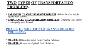
SlideShare a Scribd company logo
1 of 38
Download to read offline
UNIT 3
TRANSPORTATION
BY: ABHISHEK KUMAR
ASSISTANT PROFESSOR
N.M.S.N.DASSPG COLLEGE
BADAUN
WHAT IS TRANSPORTATION PROBLEM ?
• The transportation problem is a special type of linear programming
problem where the objective is to minimize the cost of distributing a
product from a number of sources or origins to a number
of destinations.
• Because of its special structure, the usual simplex method is not
suitable for solving transportation problems. These problems require a
special method of solution.
AIM OF TRANSPORTATION PROBLEM:
• To find out the optimum transportation schedule keeping in mind cost of
Transportation to be minimized.
• The origin of a transportation problem is the location from which shipments
are despatched.
• The destination of a transportation problem is the location to which
shipments are transported.
• The unit transportationcost is the cost of transporting one unit of the
consignment from an origin to a destination
• Determination of a transportation plan of a single commodity
• From a number of sources
• To a number of destinations,
• Such that total cost of transportation id minimized.
OBJECTIVES OF TRANSPORTATION
PROBLEM
• It is used to compute transportation routes in such a way as to minimize
transportation cost for finding out locations of warehouses.
• It is used to find out locations of transportation corporations depots where
insignificant total cost difference may not matter.
• Minimize shipping costs from factories to warehouses(or from warehouses to retail
outlets).
• Determine lowest cost location for new factory, warehouse, office ,or other
outlet facility.
• Find minimum cost production schedule that satisfies firms demand and production
limitations.
APPLICATIONS OF TRANSPORTATION
• The transportation problem is one of the most frequently encountered application in
real life situations and is a special type of linear programming problem.
• The transportation problem indicatesthe amount of consignment to be transported
from various origins to different destinations so that the total transportation cost is
minimized without violating the availability constraints and the requirement
constraints.
CONCLUSION
TWO TYPES OF TRANSPORTATION
PROBLEM:-
• BALANCED TRANSPORTATIONPROBLEM:- Where the total supply
equally total demand.
• UNBALANCED TRANSPORTATIONPROBLEM:- Where the total supply
is not equally total demand.
PHASES OF SOLUTION OF TRANSPORTATION
PROBLEM:-
▪ PHASE I:- Obtains the Initial Basic Feasible Solution.
▪ PHASE II:- Obtains the Optimal Basic Solution.
INITIAL BASIC FEASIBLE
SOLUTION:-
▪ NORTH-WEST CORNER RULE(NWCR)
▪ LEAST COST METHOD(LCM)
▪ VOGLE APPROXIMATION METHOD(VAM)
OPTIMUM BASIC SOLUTION:-
▪ MODIFIED DISTRIBUTION METHOD (MODI
METHOD)
▪ STEPPING STONE METHOD
NORTH-WEST CORNER RULE (NWCR):-
• DEFINATION:- The North-West Corner Rule is a method
adopted to compute the Initial Feasible Solution of the
transportation problem. The name North-West Corner is given to
this method because the basic variables are selected from the
extreme left corner.
• It is most systematic and easiest method for obtaining Initial
Feasible Basic Solution.
STEPS IN NORTH-WEST CORNER METHOD
▪ STEP 1:- Select the upper left (north-west) cell of the transportation
matrix and allocate minimum of supply and demand, i.e min(A1,B1)
value in that cell.
▪ STEP2:-
➢IfA1<B1, then allocation made is equal to the supply available at the
first source(A1 in first row), then move vertically down to the cell (2,1).
➢If A1>B1, then allocation made is equal to demand of the first
destination (B1 in first column), then move horizontally to the cell (1,2).
➢IfA1=B1, then allocate the value ofA1 or B1and then move to cell
(2,2).
▪ STEP3:- Continue the process until an allocation is made in the south-
east corner cell of the transportation table.
In the table, three sourcesA,B and C with the Production Capacity of 50units, 40units, 60
units of product respectively is given. Every day the demand of three retailers D,E,F is to
be furnished with at least 20units, 95units and 35units of product respectively. The
transportation costs are also given in the matrix.
Step 1:- Check whether Total Demand is equal to Total Supply. In case the demand is more
then supply, then dummy origin is added to the table. The cost associated with the dummy
origin will be zero.
Step 2:- Select the North-West or Extreme left corner of the matrix, assign as many units as
possible to cellAD, within the supply and demand constraints. Such as 20units are assigned
to the first cell, that satisfies the demand of destination D while the supply is in Surplus.
Now Assign 30 units to the cellAE. Since 30units are available with the sourceA, the
supply gets fully saturated.
SOURCE TO D E F SUPPLY
A 5 8 4 50
B 6 6 3 40
C 3 9 6 60
DEMAND 20 95 35 150/150
STEP 3:- Now move vertically, and assign 40 units to cell BE. The
supply of source B also gets fully saturated. Again move vertically,
assign 25units to cell CE, demand of destination E is fulfilled.
Move horizontally in the matrix and assign 35units to cell CF, both
the demand and supply of origin and destination get saturated. Now
Total Cost can be computed.
Total Cost can be computed by multiplying the units assigned to
each cell with the concerned transportation cost.
INTIAL TRANSPORTATION COST
TOTAL COST = (20*5)+(30*8)+(40*6)+(25*9)+(35*6)= Rs 1015.
SOURCES / TO D E F SUPPLY
A 5 (20) 8 (30) 4 50
B 6 6 (40) 3 40
C 3 9 (25) 6 (35) 60
DEMAND 20 95 35 150/150
LEASTCOST METHOD
USES OF LEAST COSTMETHOD
TRANPORTATION PROBLEM(BALANCED)
TRANPORTATION PROBLEM(UNBALANCED)
LEAST COST METHOD
Contents
Destination constraints:
Cost As A Priority
Solve the Problem
Supply constraints:
Constraints
LEAST COST METHOD
1 FINANCIALANALYSIS
2 ECONOMIC ANALYSIS
3 RISK ASSESSMENT
4 TRANPORTATION
5 ENVIRONMENT
WHERE LEAST COST METHOD IS USED
TRANSPORTATION PROBLEM WITH BALANCED SITUATIONS
ASSUMING
THEM
INDUSTRIES
ASSUMING THEM STORES
BALANCED
COST
1 The minimum cost in the matrix is Rs 3, but there is a tie in the cell BF, and CD, now the question arises in which cell we
shall allocate. Generally, the cost where maximum quantity can be assigned should be chosen to obtain the better initial
solution. Therefore, 35 units shall be assigned to the cell BF.
5
Again the minimum cost in the matrix is Rs 3. Therefore, 20 units shall be assigned to the cell CD. With this, the demand of
retailer D gets fulfilled. Only 40 units are left with the source C.
40
The next minimum cost is 8, assign 50 units to the cellAE. The supply of sourceAgets saturated.
The next minimum cost is Rs 9; we shall assign 40 units to the cell CE. With his both the demand and supply of all the
sources and origins gets saturated.
Total Cost = 50*8 + 5*6 + 35*3 +20*3 +40*9 = Rs 955.
The total cost can be calculated by multiplying the assigned
quantity with the concerned cost of the cell. Therefore,
Example of Unbalanced Transportation Problem
Plant Warehouse Supply
W1 W2 W3
A 28 17 26 500
B 19 12 16 300
Demand 250 250 500
The total demand is 1000, whereas the total supply is 800.
Si<Dj
Total supply < total demand.
Plant Warehouse Supply
W1 W2 W3
A 28 17 26 500
B 19 12 16 300
Unsatisfied demand 0 0 0 200
Demand 250 250 500 1000
VOGEL APPROXIMATION METHOD
(VAM METHOD)
The Vogel Approximation Method is an improved version of
the Minimum Cell Cost Method and the Northwest Corner
Method that in general produces better initial basic feasible
solution, that report a smaller value in the objective
(minimization) function of a balanced Transportation Problem.
(sum of the supply = sum of the demand).
Applying the V
ogel Approximation Method requires the
following STEPS:
• Step 1: Determine a penalty cost for each row (column) by
subtracting the lowest unit cell cost in the row (column) from
the next lowest unit cell cost in the same row (column).
• Step 2: Identify the row or column with the greatest penalty cost. Break the
ties arbitrarily (if there are any). Allocate as much as possible to the variable
with the lowest unit cost in the selected row or column. Adjust the supply and
demand and cross out the row or column that is already satisfied. If a row and
column are satisfied simultaneously, only cross out one of the two and allocate
a supply or demand of zero to the one that remains.
• Step 3:
• If there is exactly one row or column left with a supply or demand of zero,
stop.
• If there is one row (column) left with a positive supply (demand), determine
the basic variables in the row (column) using the Minimum Cell Cost Method.
Stop.
• If all of the rows and columns that were not crossed out have zero supply and
demand (remaining), determine the basic zero variables using the Minimum
Cell Cost Method. Stop.
• In any other case, continue with Step 1.
The concept of Vogel’s Approximation Method can be well understood
through an ILLUSTRATION given below:
• First of all the difference between two least cost cells are calculated for
each row and column, which can be seen in the iteration given for each
row and column. Then the largest difference is selected, which is 4 in this
case. So, allocate 20 units to cell BD, since the minimum cost is to be
chosen for the allocation. Now, only 20 units are left with the source B.
• Column D is deleted, again the difference between the least cost cells
is calculated for each row and column, as seen in the iteration below.
The largest difference value comes to be 3, so allocate 35 units to cell
AF and 15 units to the cell AE. With this, the Supply and demand of
source A and origin F gets saturated, so delete both the row A and
Column F.
• Now, single column E is left, since no difference can be found out, so
allocate 60 units to the cell CE and 20 units to cell BE, as only 20
units are left with source B. Hence the demand and supply are
completely met.
• Now the total cost can be computed, by multiplying the units
assigned to each cell with the cost concerned. Therefore,
• Total Cost = 20*3 + 35*1 + 15*4 + 60*4 + 20*8 = Rs 555
• Note: Vogel’s Approximation Method is also called as Penalty
Method because the difference costs chosen are nothing but the
penalties of not choosing the least cost routes.
MODI METHOD(Modified Distribution Method)
• 1. Determine an initial basicfeasiblesolution using any one of the three methods given below:
• North West CornerMethod
• Matrix MinimumMethod
• VogelApproximationMethod
• 2. Determine the values of dual variables,ui and vj, using ui + vj = cij
• 3. Computethe opportunitycost using cij – ( ui + vj ).
• 4. Check the sign of each opportunitycost. If the opportunitycosts of all the unoccupied cells are either
positiveor zero, the given solutionis the optimal solution.On the other hand, if one or more unoccupied cell
has negativeopportunitycost, the given solutionis not an optimal solutionand further savingsin
transportation cost are possible.
• 5. Select the unoccupied cellwith the smallest negativeopportunitycost as the cell to be includedin the
next solution.
• 6. Draw a closed path or loop for the unoccupied cell selected in the previous step. Please note that the right
angle turn in this path is permittedonly at occupied cells and at the original unoccupied cell.
• 7. Assign alternateplus and minus signs at the unoccupied cells on the corner points of the closed path with
a plus sign at the cell being evaluated.
• 8. Determine the maximum number of units that shouldbe shipped to this unoccupied cell. The smallest
valuewith a negativepositionon the closed path indicatesthe number of units that can be shipped to the
entering cell. Now, add this quantityto all the cells on the corner pointsof the closed path marked with plus
signs, and subtract it from those cells marked with minus signs. In this way, an unoccupied cell becomes an
occupied cell.
Distribution centre
D1 D2 D3 D4 Supply
Plant
P1 19 30 50 12 7
P2 70 30 40 60 10
P3 40 10 60 20 18
Requireme
nt
5 8 7 15
onsider the transportation problem presented in the
following table.
Distribution centre
D1 D2 D3 D4 Supply
Plant P1 19 30 50 7
P2 30 60 10
P3 60 18
Require
= 2ment
5 8 7 15
An initial basic feasible solution is obtained by Matrix
Minimum Method and is shown in table 1.
Table 1
Initial basic feasible solution
12 X 7 + 70 X 3 + 40 X 7 + 40 X 2 + 10 X 8 + 20 X 8 = Rs.
894.
Calculating ui and vj using ui + vj = cij
Substituting u1 = 0, we get
u1 + v4 = c14
c34
c32
c31
⇒ 0 + v4 = 12 or v4 = 12
⇒ u3 + 12 = 20 or u3 = 8
⇒ 8 + v2 = 10 or v2 = 2
⇒ 8 + v1 = 40 or v1 = 32
u3 + v4 =
u3 + v2 =
u3 + v1 =
u2 + v1 = c21 ⇒ u2 + 32 = 70 or u2 = 38
u2 + v3 = c23 ⇒ 38 + v3 = 40 or v3 = 2
Distribution centre
D1 D2 D3 D4 Supply ui
Plant P1 19 30 50 7 0
P2 30 60 10 38
P3 60 18 8
Requi
remen
t
5 8 7 15
vj 32 2 2 12
Unoccupied cells Opportunity cost
(P1, D1) c11 – ( u1 + v1 ) = 19 – (0 + 32) = –13
(P1, D2) c12 – ( u1 + v2 ) = 30 – (0 + 2) = 28
(P1, D3) c13 – ( u1 + v3 ) = 50 – (0 + 2) = 48
(P2, D2) c22 – ( u2 + v2 ) = 30 – (38 + 2) = –10
(P2, D4) c14 – ( u2 + v4 ) = 60 – (38 + 12) = 10
(P3, D3) c33 – ( u3 + v3 ) = 60 – (8 + 2) = 50
Calculating opportunity cost using cij – ( ui + vj )
Distribution centre
D1 D2 D3 D4 Supply ui
Plant P1 7 0
P2 10 38
P3 18 8
Requiremen
t
5 8 7 15
vj 32 2 2 12
Now choose the smallest (most) negative value from
opportunity cost (i.e., –13) and draw a closed path
from P1D1. The following table shows the closed path.
Table 4
Choose the smallest value with a negative position on
the closed path(i.e., 2), it indicates the number of units
that can be shipped to the entering cell. Now add this
quantity to all the cells on the corner points of the
closed path marked with plus signs and subtract it from
those cells marked with minus signs. In this way, an
unoccupied cell becomes an occupied cell.
Now again calculate the values for ui & vj and
opportunity cost. The resulting matrix is shown below.
Table 5
Distribution centre
D1 D2 D3 D4 Supply ui
Plant P1 7 0
P2 10 51
P3 18 8
Requir
ement
5 8 7 15
vj 19 2 –11 12
Choose the smallest (most) negative value from
opportunity cost (i.e., –23). Now draw a closed path
from P2D2 .
Now again calculate the values for ui & vj and opportunity
cost
Distribution centre
D1 D2 D3 D4 Supply ui
Plant P1 7 0
P2 10 28
P3 18 8
Requi
remen
t
5 8 7 15
vj 19 2 12 12
Since all the current opportunity costs are non–negative,
this is the optimal solution. The minimum transportation
cost is: 19 X 5 + 12 X 2 + 30 X 3 + 40 X 7 + 10 X 5 + 20 X
13 = Rs. 799

More Related Content

Similar to O.R UNIT 3.pdf

QA CHAPTER III and IV(1)(1).pdf
QA CHAPTER III and IV(1)(1).pdfQA CHAPTER III and IV(1)(1).pdf
QA CHAPTER III and IV(1)(1).pdfTeshome48
 
transporation problem
transporation problemtransporation problem
transporation problemVivek Lohani
 
chapter 3.pptx
chapter 3.pptxchapter 3.pptx
chapter 3.pptxDejeneDay
 
LP network chapter 5 transportation and assignment problem
LP  network chapter 5 transportation and assignment problemLP  network chapter 5 transportation and assignment problem
LP network chapter 5 transportation and assignment problemHarun Al-Rasyid Lubis
 
Transportation model
Transportation modelTransportation model
Transportation modelshakila haque
 
Linear Programming.pptx
Linear Programming.pptxLinear Programming.pptx
Linear Programming.pptxDrBabinDhasD
 
03-Unit Three -OR.pptx
03-Unit Three -OR.pptx03-Unit Three -OR.pptx
03-Unit Three -OR.pptxAbdiMuceeTube
 
Transportatopn problm
Transportatopn problmTransportatopn problm
Transportatopn problmAnshul Singh
 
Mba i qt unit-1.2_transportation, assignment and transshipment problems
Mba i qt unit-1.2_transportation, assignment and transshipment problemsMba i qt unit-1.2_transportation, assignment and transshipment problems
Mba i qt unit-1.2_transportation, assignment and transshipment problemsRai University
 
Transportation problem
Transportation problemTransportation problem
Transportation problemShubhagata Roy
 
Transportation problem ppt
Transportation problem pptTransportation problem ppt
Transportation problem pptDr T.Sivakami
 
MODI Method (Operations Research)
MODI Method (Operations Research) MODI Method (Operations Research)
MODI Method (Operations Research) Nilraj Vasandia
 
Transportationproblem 111218100045-phpapp01
Transportationproblem 111218100045-phpapp01Transportationproblem 111218100045-phpapp01
Transportationproblem 111218100045-phpapp01RAJUMARU3
 
Top school in delhi ncr
Top school in delhi ncrTop school in delhi ncr
Top school in delhi ncrEdhole.com
 

Similar to O.R UNIT 3.pdf (20)

QA CHAPTER III and IV(1)(1).pdf
QA CHAPTER III and IV(1)(1).pdfQA CHAPTER III and IV(1)(1).pdf
QA CHAPTER III and IV(1)(1).pdf
 
07. Transportation Problem.pptx
07. Transportation Problem.pptx07. Transportation Problem.pptx
07. Transportation Problem.pptx
 
OR 14 15-unit_2
OR 14 15-unit_2OR 14 15-unit_2
OR 14 15-unit_2
 
transporation problem
transporation problemtransporation problem
transporation problem
 
LEAST COST METHOD
LEAST COST METHOD LEAST COST METHOD
LEAST COST METHOD
 
5. transportation problems
5. transportation problems5. transportation problems
5. transportation problems
 
Transportation problem
Transportation problemTransportation problem
Transportation problem
 
chapter 3.pptx
chapter 3.pptxchapter 3.pptx
chapter 3.pptx
 
LP network chapter 5 transportation and assignment problem
LP  network chapter 5 transportation and assignment problemLP  network chapter 5 transportation and assignment problem
LP network chapter 5 transportation and assignment problem
 
Transportation model
Transportation modelTransportation model
Transportation model
 
Linear Programming.pptx
Linear Programming.pptxLinear Programming.pptx
Linear Programming.pptx
 
03-Unit Three -OR.pptx
03-Unit Three -OR.pptx03-Unit Three -OR.pptx
03-Unit Three -OR.pptx
 
Transportatopn problm
Transportatopn problmTransportatopn problm
Transportatopn problm
 
Mba i qt unit-1.2_transportation, assignment and transshipment problems
Mba i qt unit-1.2_transportation, assignment and transshipment problemsMba i qt unit-1.2_transportation, assignment and transshipment problems
Mba i qt unit-1.2_transportation, assignment and transshipment problems
 
Transportation problem
Transportation problemTransportation problem
Transportation problem
 
Transportation problem ppt
Transportation problem pptTransportation problem ppt
Transportation problem ppt
 
MODI Method (Operations Research)
MODI Method (Operations Research) MODI Method (Operations Research)
MODI Method (Operations Research)
 
Operations Research Project
Operations Research ProjectOperations Research Project
Operations Research Project
 
Transportationproblem 111218100045-phpapp01
Transportationproblem 111218100045-phpapp01Transportationproblem 111218100045-phpapp01
Transportationproblem 111218100045-phpapp01
 
Top school in delhi ncr
Top school in delhi ncrTop school in delhi ncr
Top school in delhi ncr
 

Recently uploaded

“Oh GOSH! Reflecting on Hackteria's Collaborative Practices in a Global Do-It...
“Oh GOSH! Reflecting on Hackteria's Collaborative Practices in a Global Do-It...“Oh GOSH! Reflecting on Hackteria's Collaborative Practices in a Global Do-It...
“Oh GOSH! Reflecting on Hackteria's Collaborative Practices in a Global Do-It...Marc Dusseiller Dusjagr
 
mini mental status format.docx
mini    mental       status     format.docxmini    mental       status     format.docx
mini mental status format.docxPoojaSen20
 
Incoming and Outgoing Shipments in 1 STEP Using Odoo 17
Incoming and Outgoing Shipments in 1 STEP Using Odoo 17Incoming and Outgoing Shipments in 1 STEP Using Odoo 17
Incoming and Outgoing Shipments in 1 STEP Using Odoo 17Celine George
 
_Math 4-Q4 Week 5.pptx Steps in Collecting Data
_Math 4-Q4 Week 5.pptx Steps in Collecting Data_Math 4-Q4 Week 5.pptx Steps in Collecting Data
_Math 4-Q4 Week 5.pptx Steps in Collecting DataJhengPantaleon
 
How to Make a Pirate ship Primary Education.pptx
How to Make a Pirate ship Primary Education.pptxHow to Make a Pirate ship Primary Education.pptx
How to Make a Pirate ship Primary Education.pptxmanuelaromero2013
 
Hybridoma Technology ( Production , Purification , and Application )
Hybridoma Technology  ( Production , Purification , and Application  ) Hybridoma Technology  ( Production , Purification , and Application  )
Hybridoma Technology ( Production , Purification , and Application ) Sakshi Ghasle
 
Kisan Call Centre - To harness potential of ICT in Agriculture by answer farm...
Kisan Call Centre - To harness potential of ICT in Agriculture by answer farm...Kisan Call Centre - To harness potential of ICT in Agriculture by answer farm...
Kisan Call Centre - To harness potential of ICT in Agriculture by answer farm...Krashi Coaching
 
Crayon Activity Handout For the Crayon A
Crayon Activity Handout For the Crayon ACrayon Activity Handout For the Crayon A
Crayon Activity Handout For the Crayon AUnboundStockton
 
SOCIAL AND HISTORICAL CONTEXT - LFTVD.pptx
SOCIAL AND HISTORICAL CONTEXT - LFTVD.pptxSOCIAL AND HISTORICAL CONTEXT - LFTVD.pptx
SOCIAL AND HISTORICAL CONTEXT - LFTVD.pptxiammrhaywood
 
A Critique of the Proposed National Education Policy Reform
A Critique of the Proposed National Education Policy ReformA Critique of the Proposed National Education Policy Reform
A Critique of the Proposed National Education Policy ReformChameera Dedduwage
 
Software Engineering Methodologies (overview)
Software Engineering Methodologies (overview)Software Engineering Methodologies (overview)
Software Engineering Methodologies (overview)eniolaolutunde
 
Presiding Officer Training module 2024 lok sabha elections
Presiding Officer Training module 2024 lok sabha electionsPresiding Officer Training module 2024 lok sabha elections
Presiding Officer Training module 2024 lok sabha electionsanshu789521
 
Accessible design: Minimum effort, maximum impact
Accessible design: Minimum effort, maximum impactAccessible design: Minimum effort, maximum impact
Accessible design: Minimum effort, maximum impactdawncurless
 
URLs and Routing in the Odoo 17 Website App
URLs and Routing in the Odoo 17 Website AppURLs and Routing in the Odoo 17 Website App
URLs and Routing in the Odoo 17 Website AppCeline George
 
PSYCHIATRIC History collection FORMAT.pptx
PSYCHIATRIC   History collection FORMAT.pptxPSYCHIATRIC   History collection FORMAT.pptx
PSYCHIATRIC History collection FORMAT.pptxPoojaSen20
 
MENTAL STATUS EXAMINATION format.docx
MENTAL     STATUS EXAMINATION format.docxMENTAL     STATUS EXAMINATION format.docx
MENTAL STATUS EXAMINATION format.docxPoojaSen20
 
POINT- BIOCHEMISTRY SEM 2 ENZYMES UNIT 5.pptx
POINT- BIOCHEMISTRY SEM 2 ENZYMES UNIT 5.pptxPOINT- BIOCHEMISTRY SEM 2 ENZYMES UNIT 5.pptx
POINT- BIOCHEMISTRY SEM 2 ENZYMES UNIT 5.pptxSayali Powar
 
CARE OF CHILD IN INCUBATOR..........pptx
CARE OF CHILD IN INCUBATOR..........pptxCARE OF CHILD IN INCUBATOR..........pptx
CARE OF CHILD IN INCUBATOR..........pptxGaneshChakor2
 

Recently uploaded (20)

“Oh GOSH! Reflecting on Hackteria's Collaborative Practices in a Global Do-It...
“Oh GOSH! Reflecting on Hackteria's Collaborative Practices in a Global Do-It...“Oh GOSH! Reflecting on Hackteria's Collaborative Practices in a Global Do-It...
“Oh GOSH! Reflecting on Hackteria's Collaborative Practices in a Global Do-It...
 
mini mental status format.docx
mini    mental       status     format.docxmini    mental       status     format.docx
mini mental status format.docx
 
Incoming and Outgoing Shipments in 1 STEP Using Odoo 17
Incoming and Outgoing Shipments in 1 STEP Using Odoo 17Incoming and Outgoing Shipments in 1 STEP Using Odoo 17
Incoming and Outgoing Shipments in 1 STEP Using Odoo 17
 
_Math 4-Q4 Week 5.pptx Steps in Collecting Data
_Math 4-Q4 Week 5.pptx Steps in Collecting Data_Math 4-Q4 Week 5.pptx Steps in Collecting Data
_Math 4-Q4 Week 5.pptx Steps in Collecting Data
 
How to Make a Pirate ship Primary Education.pptx
How to Make a Pirate ship Primary Education.pptxHow to Make a Pirate ship Primary Education.pptx
How to Make a Pirate ship Primary Education.pptx
 
Hybridoma Technology ( Production , Purification , and Application )
Hybridoma Technology  ( Production , Purification , and Application  ) Hybridoma Technology  ( Production , Purification , and Application  )
Hybridoma Technology ( Production , Purification , and Application )
 
Kisan Call Centre - To harness potential of ICT in Agriculture by answer farm...
Kisan Call Centre - To harness potential of ICT in Agriculture by answer farm...Kisan Call Centre - To harness potential of ICT in Agriculture by answer farm...
Kisan Call Centre - To harness potential of ICT in Agriculture by answer farm...
 
Crayon Activity Handout For the Crayon A
Crayon Activity Handout For the Crayon ACrayon Activity Handout For the Crayon A
Crayon Activity Handout For the Crayon A
 
SOCIAL AND HISTORICAL CONTEXT - LFTVD.pptx
SOCIAL AND HISTORICAL CONTEXT - LFTVD.pptxSOCIAL AND HISTORICAL CONTEXT - LFTVD.pptx
SOCIAL AND HISTORICAL CONTEXT - LFTVD.pptx
 
A Critique of the Proposed National Education Policy Reform
A Critique of the Proposed National Education Policy ReformA Critique of the Proposed National Education Policy Reform
A Critique of the Proposed National Education Policy Reform
 
Software Engineering Methodologies (overview)
Software Engineering Methodologies (overview)Software Engineering Methodologies (overview)
Software Engineering Methodologies (overview)
 
Presiding Officer Training module 2024 lok sabha elections
Presiding Officer Training module 2024 lok sabha electionsPresiding Officer Training module 2024 lok sabha elections
Presiding Officer Training module 2024 lok sabha elections
 
Accessible design: Minimum effort, maximum impact
Accessible design: Minimum effort, maximum impactAccessible design: Minimum effort, maximum impact
Accessible design: Minimum effort, maximum impact
 
URLs and Routing in the Odoo 17 Website App
URLs and Routing in the Odoo 17 Website AppURLs and Routing in the Odoo 17 Website App
URLs and Routing in the Odoo 17 Website App
 
Model Call Girl in Tilak Nagar Delhi reach out to us at 🔝9953056974🔝
Model Call Girl in Tilak Nagar Delhi reach out to us at 🔝9953056974🔝Model Call Girl in Tilak Nagar Delhi reach out to us at 🔝9953056974🔝
Model Call Girl in Tilak Nagar Delhi reach out to us at 🔝9953056974🔝
 
PSYCHIATRIC History collection FORMAT.pptx
PSYCHIATRIC   History collection FORMAT.pptxPSYCHIATRIC   History collection FORMAT.pptx
PSYCHIATRIC History collection FORMAT.pptx
 
MENTAL STATUS EXAMINATION format.docx
MENTAL     STATUS EXAMINATION format.docxMENTAL     STATUS EXAMINATION format.docx
MENTAL STATUS EXAMINATION format.docx
 
POINT- BIOCHEMISTRY SEM 2 ENZYMES UNIT 5.pptx
POINT- BIOCHEMISTRY SEM 2 ENZYMES UNIT 5.pptxPOINT- BIOCHEMISTRY SEM 2 ENZYMES UNIT 5.pptx
POINT- BIOCHEMISTRY SEM 2 ENZYMES UNIT 5.pptx
 
CARE OF CHILD IN INCUBATOR..........pptx
CARE OF CHILD IN INCUBATOR..........pptxCARE OF CHILD IN INCUBATOR..........pptx
CARE OF CHILD IN INCUBATOR..........pptx
 
Staff of Color (SOC) Retention Efforts DDSD
Staff of Color (SOC) Retention Efforts DDSDStaff of Color (SOC) Retention Efforts DDSD
Staff of Color (SOC) Retention Efforts DDSD
 

O.R UNIT 3.pdf

  • 1. UNIT 3 TRANSPORTATION BY: ABHISHEK KUMAR ASSISTANT PROFESSOR N.M.S.N.DASSPG COLLEGE BADAUN
  • 2. WHAT IS TRANSPORTATION PROBLEM ? • The transportation problem is a special type of linear programming problem where the objective is to minimize the cost of distributing a product from a number of sources or origins to a number of destinations. • Because of its special structure, the usual simplex method is not suitable for solving transportation problems. These problems require a special method of solution.
  • 3. AIM OF TRANSPORTATION PROBLEM: • To find out the optimum transportation schedule keeping in mind cost of Transportation to be minimized. • The origin of a transportation problem is the location from which shipments are despatched. • The destination of a transportation problem is the location to which shipments are transported. • The unit transportationcost is the cost of transporting one unit of the consignment from an origin to a destination
  • 4. • Determination of a transportation plan of a single commodity • From a number of sources • To a number of destinations, • Such that total cost of transportation id minimized. OBJECTIVES OF TRANSPORTATION PROBLEM
  • 5. • It is used to compute transportation routes in such a way as to minimize transportation cost for finding out locations of warehouses. • It is used to find out locations of transportation corporations depots where insignificant total cost difference may not matter. • Minimize shipping costs from factories to warehouses(or from warehouses to retail outlets). • Determine lowest cost location for new factory, warehouse, office ,or other outlet facility. • Find minimum cost production schedule that satisfies firms demand and production limitations. APPLICATIONS OF TRANSPORTATION
  • 6. • The transportation problem is one of the most frequently encountered application in real life situations and is a special type of linear programming problem. • The transportation problem indicatesthe amount of consignment to be transported from various origins to different destinations so that the total transportation cost is minimized without violating the availability constraints and the requirement constraints. CONCLUSION
  • 7. TWO TYPES OF TRANSPORTATION PROBLEM:- • BALANCED TRANSPORTATIONPROBLEM:- Where the total supply equally total demand. • UNBALANCED TRANSPORTATIONPROBLEM:- Where the total supply is not equally total demand. PHASES OF SOLUTION OF TRANSPORTATION PROBLEM:- ▪ PHASE I:- Obtains the Initial Basic Feasible Solution. ▪ PHASE II:- Obtains the Optimal Basic Solution.
  • 8. INITIAL BASIC FEASIBLE SOLUTION:- ▪ NORTH-WEST CORNER RULE(NWCR) ▪ LEAST COST METHOD(LCM) ▪ VOGLE APPROXIMATION METHOD(VAM) OPTIMUM BASIC SOLUTION:- ▪ MODIFIED DISTRIBUTION METHOD (MODI METHOD) ▪ STEPPING STONE METHOD
  • 9. NORTH-WEST CORNER RULE (NWCR):- • DEFINATION:- The North-West Corner Rule is a method adopted to compute the Initial Feasible Solution of the transportation problem. The name North-West Corner is given to this method because the basic variables are selected from the extreme left corner. • It is most systematic and easiest method for obtaining Initial Feasible Basic Solution.
  • 10. STEPS IN NORTH-WEST CORNER METHOD ▪ STEP 1:- Select the upper left (north-west) cell of the transportation matrix and allocate minimum of supply and demand, i.e min(A1,B1) value in that cell. ▪ STEP2:- ➢IfA1<B1, then allocation made is equal to the supply available at the first source(A1 in first row), then move vertically down to the cell (2,1). ➢If A1>B1, then allocation made is equal to demand of the first destination (B1 in first column), then move horizontally to the cell (1,2). ➢IfA1=B1, then allocate the value ofA1 or B1and then move to cell (2,2). ▪ STEP3:- Continue the process until an allocation is made in the south- east corner cell of the transportation table.
  • 11. In the table, three sourcesA,B and C with the Production Capacity of 50units, 40units, 60 units of product respectively is given. Every day the demand of three retailers D,E,F is to be furnished with at least 20units, 95units and 35units of product respectively. The transportation costs are also given in the matrix. Step 1:- Check whether Total Demand is equal to Total Supply. In case the demand is more then supply, then dummy origin is added to the table. The cost associated with the dummy origin will be zero. Step 2:- Select the North-West or Extreme left corner of the matrix, assign as many units as possible to cellAD, within the supply and demand constraints. Such as 20units are assigned to the first cell, that satisfies the demand of destination D while the supply is in Surplus. Now Assign 30 units to the cellAE. Since 30units are available with the sourceA, the supply gets fully saturated. SOURCE TO D E F SUPPLY A 5 8 4 50 B 6 6 3 40 C 3 9 6 60 DEMAND 20 95 35 150/150
  • 12. STEP 3:- Now move vertically, and assign 40 units to cell BE. The supply of source B also gets fully saturated. Again move vertically, assign 25units to cell CE, demand of destination E is fulfilled. Move horizontally in the matrix and assign 35units to cell CF, both the demand and supply of origin and destination get saturated. Now Total Cost can be computed. Total Cost can be computed by multiplying the units assigned to each cell with the concerned transportation cost. INTIAL TRANSPORTATION COST TOTAL COST = (20*5)+(30*8)+(40*6)+(25*9)+(35*6)= Rs 1015. SOURCES / TO D E F SUPPLY A 5 (20) 8 (30) 4 50 B 6 6 (40) 3 40 C 3 9 (25) 6 (35) 60 DEMAND 20 95 35 150/150
  • 13. LEASTCOST METHOD USES OF LEAST COSTMETHOD TRANPORTATION PROBLEM(BALANCED) TRANPORTATION PROBLEM(UNBALANCED) LEAST COST METHOD Contents
  • 14. Destination constraints: Cost As A Priority Solve the Problem Supply constraints: Constraints LEAST COST METHOD
  • 15. 1 FINANCIALANALYSIS 2 ECONOMIC ANALYSIS 3 RISK ASSESSMENT 4 TRANPORTATION 5 ENVIRONMENT WHERE LEAST COST METHOD IS USED
  • 16. TRANSPORTATION PROBLEM WITH BALANCED SITUATIONS ASSUMING THEM INDUSTRIES ASSUMING THEM STORES BALANCED COST
  • 17. 1 The minimum cost in the matrix is Rs 3, but there is a tie in the cell BF, and CD, now the question arises in which cell we shall allocate. Generally, the cost where maximum quantity can be assigned should be chosen to obtain the better initial solution. Therefore, 35 units shall be assigned to the cell BF.
  • 18. 5 Again the minimum cost in the matrix is Rs 3. Therefore, 20 units shall be assigned to the cell CD. With this, the demand of retailer D gets fulfilled. Only 40 units are left with the source C.
  • 19. 40 The next minimum cost is 8, assign 50 units to the cellAE. The supply of sourceAgets saturated. The next minimum cost is Rs 9; we shall assign 40 units to the cell CE. With his both the demand and supply of all the sources and origins gets saturated.
  • 20. Total Cost = 50*8 + 5*6 + 35*3 +20*3 +40*9 = Rs 955. The total cost can be calculated by multiplying the assigned quantity with the concerned cost of the cell. Therefore,
  • 21. Example of Unbalanced Transportation Problem Plant Warehouse Supply W1 W2 W3 A 28 17 26 500 B 19 12 16 300 Demand 250 250 500 The total demand is 1000, whereas the total supply is 800. Si<Dj Total supply < total demand.
  • 22. Plant Warehouse Supply W1 W2 W3 A 28 17 26 500 B 19 12 16 300 Unsatisfied demand 0 0 0 200 Demand 250 250 500 1000
  • 23. VOGEL APPROXIMATION METHOD (VAM METHOD) The Vogel Approximation Method is an improved version of the Minimum Cell Cost Method and the Northwest Corner Method that in general produces better initial basic feasible solution, that report a smaller value in the objective (minimization) function of a balanced Transportation Problem. (sum of the supply = sum of the demand). Applying the V ogel Approximation Method requires the following STEPS: • Step 1: Determine a penalty cost for each row (column) by subtracting the lowest unit cell cost in the row (column) from the next lowest unit cell cost in the same row (column).
  • 24. • Step 2: Identify the row or column with the greatest penalty cost. Break the ties arbitrarily (if there are any). Allocate as much as possible to the variable with the lowest unit cost in the selected row or column. Adjust the supply and demand and cross out the row or column that is already satisfied. If a row and column are satisfied simultaneously, only cross out one of the two and allocate a supply or demand of zero to the one that remains. • Step 3: • If there is exactly one row or column left with a supply or demand of zero, stop. • If there is one row (column) left with a positive supply (demand), determine the basic variables in the row (column) using the Minimum Cell Cost Method. Stop. • If all of the rows and columns that were not crossed out have zero supply and demand (remaining), determine the basic zero variables using the Minimum Cell Cost Method. Stop. • In any other case, continue with Step 1.
  • 25. The concept of Vogel’s Approximation Method can be well understood through an ILLUSTRATION given below: • First of all the difference between two least cost cells are calculated for each row and column, which can be seen in the iteration given for each row and column. Then the largest difference is selected, which is 4 in this case. So, allocate 20 units to cell BD, since the minimum cost is to be chosen for the allocation. Now, only 20 units are left with the source B.
  • 26. • Column D is deleted, again the difference between the least cost cells is calculated for each row and column, as seen in the iteration below. The largest difference value comes to be 3, so allocate 35 units to cell AF and 15 units to the cell AE. With this, the Supply and demand of source A and origin F gets saturated, so delete both the row A and Column F.
  • 27. • Now, single column E is left, since no difference can be found out, so allocate 60 units to the cell CE and 20 units to cell BE, as only 20 units are left with source B. Hence the demand and supply are completely met.
  • 28. • Now the total cost can be computed, by multiplying the units assigned to each cell with the cost concerned. Therefore, • Total Cost = 20*3 + 35*1 + 15*4 + 60*4 + 20*8 = Rs 555 • Note: Vogel’s Approximation Method is also called as Penalty Method because the difference costs chosen are nothing but the penalties of not choosing the least cost routes.
  • 29. MODI METHOD(Modified Distribution Method) • 1. Determine an initial basicfeasiblesolution using any one of the three methods given below: • North West CornerMethod • Matrix MinimumMethod • VogelApproximationMethod • 2. Determine the values of dual variables,ui and vj, using ui + vj = cij • 3. Computethe opportunitycost using cij – ( ui + vj ). • 4. Check the sign of each opportunitycost. If the opportunitycosts of all the unoccupied cells are either positiveor zero, the given solutionis the optimal solution.On the other hand, if one or more unoccupied cell has negativeopportunitycost, the given solutionis not an optimal solutionand further savingsin transportation cost are possible. • 5. Select the unoccupied cellwith the smallest negativeopportunitycost as the cell to be includedin the next solution. • 6. Draw a closed path or loop for the unoccupied cell selected in the previous step. Please note that the right angle turn in this path is permittedonly at occupied cells and at the original unoccupied cell. • 7. Assign alternateplus and minus signs at the unoccupied cells on the corner points of the closed path with a plus sign at the cell being evaluated. • 8. Determine the maximum number of units that shouldbe shipped to this unoccupied cell. The smallest valuewith a negativepositionon the closed path indicatesthe number of units that can be shipped to the entering cell. Now, add this quantityto all the cells on the corner pointsof the closed path marked with plus signs, and subtract it from those cells marked with minus signs. In this way, an unoccupied cell becomes an occupied cell.
  • 30. Distribution centre D1 D2 D3 D4 Supply Plant P1 19 30 50 12 7 P2 70 30 40 60 10 P3 40 10 60 20 18 Requireme nt 5 8 7 15 onsider the transportation problem presented in the following table.
  • 31. Distribution centre D1 D2 D3 D4 Supply Plant P1 19 30 50 7 P2 30 60 10 P3 60 18 Require = 2ment 5 8 7 15 An initial basic feasible solution is obtained by Matrix Minimum Method and is shown in table 1. Table 1 Initial basic feasible solution 12 X 7 + 70 X 3 + 40 X 7 + 40 X 2 + 10 X 8 + 20 X 8 = Rs. 894.
  • 32. Calculating ui and vj using ui + vj = cij Substituting u1 = 0, we get u1 + v4 = c14 c34 c32 c31 ⇒ 0 + v4 = 12 or v4 = 12 ⇒ u3 + 12 = 20 or u3 = 8 ⇒ 8 + v2 = 10 or v2 = 2 ⇒ 8 + v1 = 40 or v1 = 32 u3 + v4 = u3 + v2 = u3 + v1 = u2 + v1 = c21 ⇒ u2 + 32 = 70 or u2 = 38 u2 + v3 = c23 ⇒ 38 + v3 = 40 or v3 = 2 Distribution centre D1 D2 D3 D4 Supply ui Plant P1 19 30 50 7 0 P2 30 60 10 38 P3 60 18 8 Requi remen t 5 8 7 15 vj 32 2 2 12
  • 33. Unoccupied cells Opportunity cost (P1, D1) c11 – ( u1 + v1 ) = 19 – (0 + 32) = –13 (P1, D2) c12 – ( u1 + v2 ) = 30 – (0 + 2) = 28 (P1, D3) c13 – ( u1 + v3 ) = 50 – (0 + 2) = 48 (P2, D2) c22 – ( u2 + v2 ) = 30 – (38 + 2) = –10 (P2, D4) c14 – ( u2 + v4 ) = 60 – (38 + 12) = 10 (P3, D3) c33 – ( u3 + v3 ) = 60 – (8 + 2) = 50 Calculating opportunity cost using cij – ( ui + vj )
  • 34. Distribution centre D1 D2 D3 D4 Supply ui Plant P1 7 0 P2 10 38 P3 18 8 Requiremen t 5 8 7 15 vj 32 2 2 12 Now choose the smallest (most) negative value from opportunity cost (i.e., –13) and draw a closed path from P1D1. The following table shows the closed path. Table 4
  • 35. Choose the smallest value with a negative position on the closed path(i.e., 2), it indicates the number of units that can be shipped to the entering cell. Now add this quantity to all the cells on the corner points of the closed path marked with plus signs and subtract it from those cells marked with minus signs. In this way, an unoccupied cell becomes an occupied cell. Now again calculate the values for ui & vj and opportunity cost. The resulting matrix is shown below. Table 5
  • 36. Distribution centre D1 D2 D3 D4 Supply ui Plant P1 7 0 P2 10 51 P3 18 8 Requir ement 5 8 7 15 vj 19 2 –11 12 Choose the smallest (most) negative value from opportunity cost (i.e., –23). Now draw a closed path from P2D2 .
  • 37. Now again calculate the values for ui & vj and opportunity cost
  • 38. Distribution centre D1 D2 D3 D4 Supply ui Plant P1 7 0 P2 10 28 P3 18 8 Requi remen t 5 8 7 15 vj 19 2 12 12 Since all the current opportunity costs are non–negative, this is the optimal solution. The minimum transportation cost is: 19 X 5 + 12 X 2 + 30 X 3 + 40 X 7 + 10 X 5 + 20 X 13 = Rs. 799